Workshop Overview
Overview
Teaching: 30 min
Exercises: 10 minQuestions
What is RNA-seq?
What data will we be using in this workshop?
Objectives
Understand the basics of RNA-seq, from sample collection through to data generation.
Learn a little bit about teh yeast data set being used in this session.
RNA-seq Workflow
Before beginning an RNA-Seq experiment, you should understand and carefully consider each step of the RNA-Seq workflow: Experimental design, Extraction, Library preparation, Sequencing, and Data analysis.
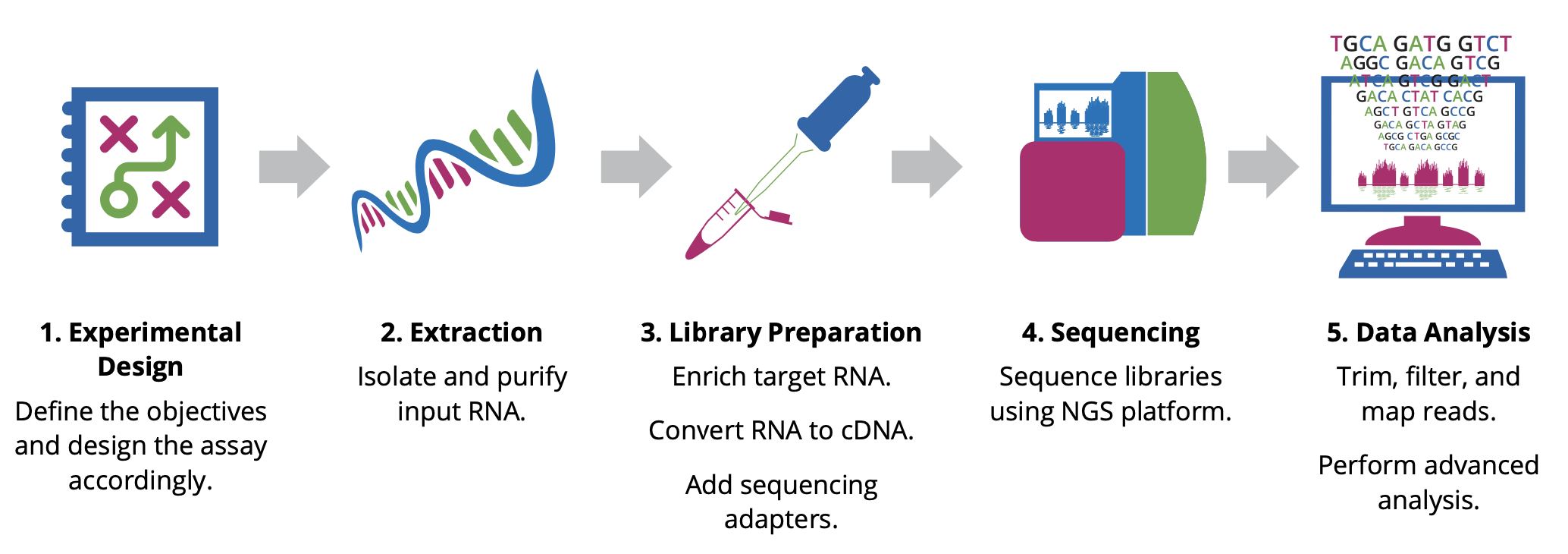
Experimental design
The design stage of your experiment is arguably the most critical step in ensuring the success of an RNA-Seq experiment. Researchers must make key decisions at the start of any NGS project, including the type of assay and the number of samples to analyze. The optimal approach will depend largely on the objectives of the experiment, hypotheses to be tested, and expected information to be gathered.
Extraction
The first step in characterizing the transcriptome involves isolating and purifying cellular RNA. The quality and quantity of the input material have a significant impact on data quality; therefore, care must be taken when isolating and preparing RNA for sequencing. Given the chemical instability of RNA, there are two major reasons for RNA degradation during experiments:
- RNA contains ribose sugar and is not stable in alkaline conditions because of the reactive hydroxyl bonds. RNA is also more prone to heat degradation than DNA.
- Ribonucleases (RNases) are ubiquitous and very stable, so avoiding them is nearly impossible. It is essential to maintain an RNase-free environment by wearing sterile disposable gloves when handling reagents and RNA samples, employing RNase inhibitors, and using DEPC-treated water instead of PCR-grade water. Additionally, proper storage of RNA is crucial to avoid RNA degradation.
In the short term, RNA may be stored in RNase-free water or TE buffer at -80°C for 1 year without degradation. For the long term, RNA samples may be stored as ethanol precipitates at -20°C. Avoid repeated freeze-thaw cycles of samples, which can lead to degradation. RNA of high integrity will maximize the likelihood of obtaining reliable and informative results.
Library Preparation
This involves generating a collection of RNA fragments that are compatible for sequencing. The process involves enrichment of target (non-ribosomal) RNA, fragmentation, reverse transcription (i.e. cDNA synthesis), and addition of sequencing adapters and amplification. The enrichment method determines which types of transcripts (e.g. mRNA, lncRNA, miRNA) will be included in the library. In addition, the cDNA synthesis step can be performed in a such a way as to maintain the original strand orientation of the transcript, generating what is known as ‘strand-specific’ or ‘directional’ libraries.
Sequencing
Parameters for sequencing—such as read length, configuration, and output—depend on the goals of your project and will influence your choice of instrument and sequencing chemistry. The main NGS technologies can be grouped into two categories: short-read (or ‘second generation’) sequencing, and long-read (or ‘third generation’) sequencing. Both have distinct benefits for RNA-Seq.
- Short-read sequencing is relatively inexpensive on a per-base basis and can generate billions of reads in a massively parallel manner, with single-end read lengths ranging between 50 and 300 bp. The high-throughput nature of this technology is ideal for quantifying the relative abundance of transcripts or identifying rare transcripts. Several platforms available on the market offer flexible outputs using roughly similar chemistry. Each cDNA fragment can be sequenced from only one end, called single-end (SE) sequencing, or both ends, called paired-end (PE) sequencing. The former is generally less expensive and faster than the latter. However, paired-end sequencing helps detect genomic rearrangements and repetitive sequence alignments better than the single- end configuration, since more information is collected from each fragment.
- Long-read sequencing can resolve inaccessible regions of the genome and read through the entire length of RNA transcripts, allowing precise determination of specific isoforms. Two of the leading long-read sequencing platform providers include Pacific Biosciences (PacBio), and Oxford Nanopore Technologies®.
However, if cost reduction is paramount and/or high data output is required, short-read sequencing is a better choice.
Data Analysis
Evaluating your data quality and extracting biologically relevant information is the final and most rewarding step in an RNA-Seq experiment. It is important to discuss your project with an experienced bioinformatician to find the best analysis pipeline for your data. One pipeline does not fit all approaches.
Exercise
Discussion: what are some possible uses of RNA-seq?
Solution
- Rank genes based on expression
- Identify differentially expressed genes after inducing a drug
- Identify novel transcripts
- Identify bacterial and eukaryotic genes in a sample
- Investigate alternative splicing and isoform usage
- De novo transcriptome assembly
- Others?
Introduction
This workshop uses the dataset from yeast RNA-seq experiment, Lee et al 2008
Yeast Dataset
- Wild-type versus RNA degradation mutants
- Subset of data (chromosome 1)
- Six samples (3 WT / 3 MT)
- Single end sequencing
Overview of Illumina Sequencing
Here is a video to illumina sequencing.
Key Points
RNA-seq is a commonly used technology for profiling the transcriptome.
There are a number of different applications for RNA-seq data - we’ll be looking at detecetign differentially expressed genes using data from an experiment involving RNA-seq data from yeast.
Quality control of the sequencing data.
Overview
Teaching: 30 min
Exercises: 0 minQuestions
What tools do we use to assess the data quality data in RNA-seq experiments?
Objectives
Learn how to assess data quality
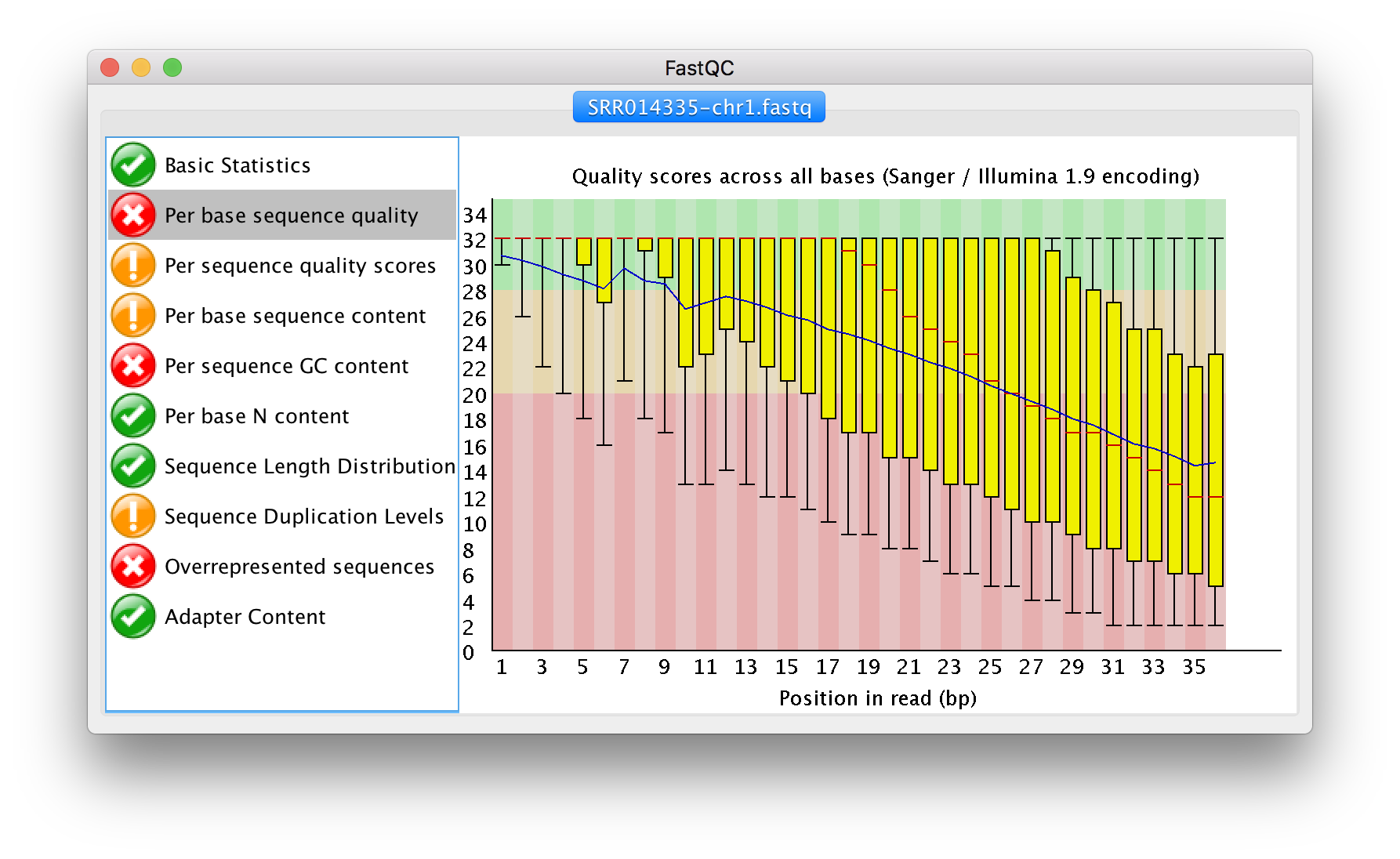
Use the FastQC application to perform quality assessment
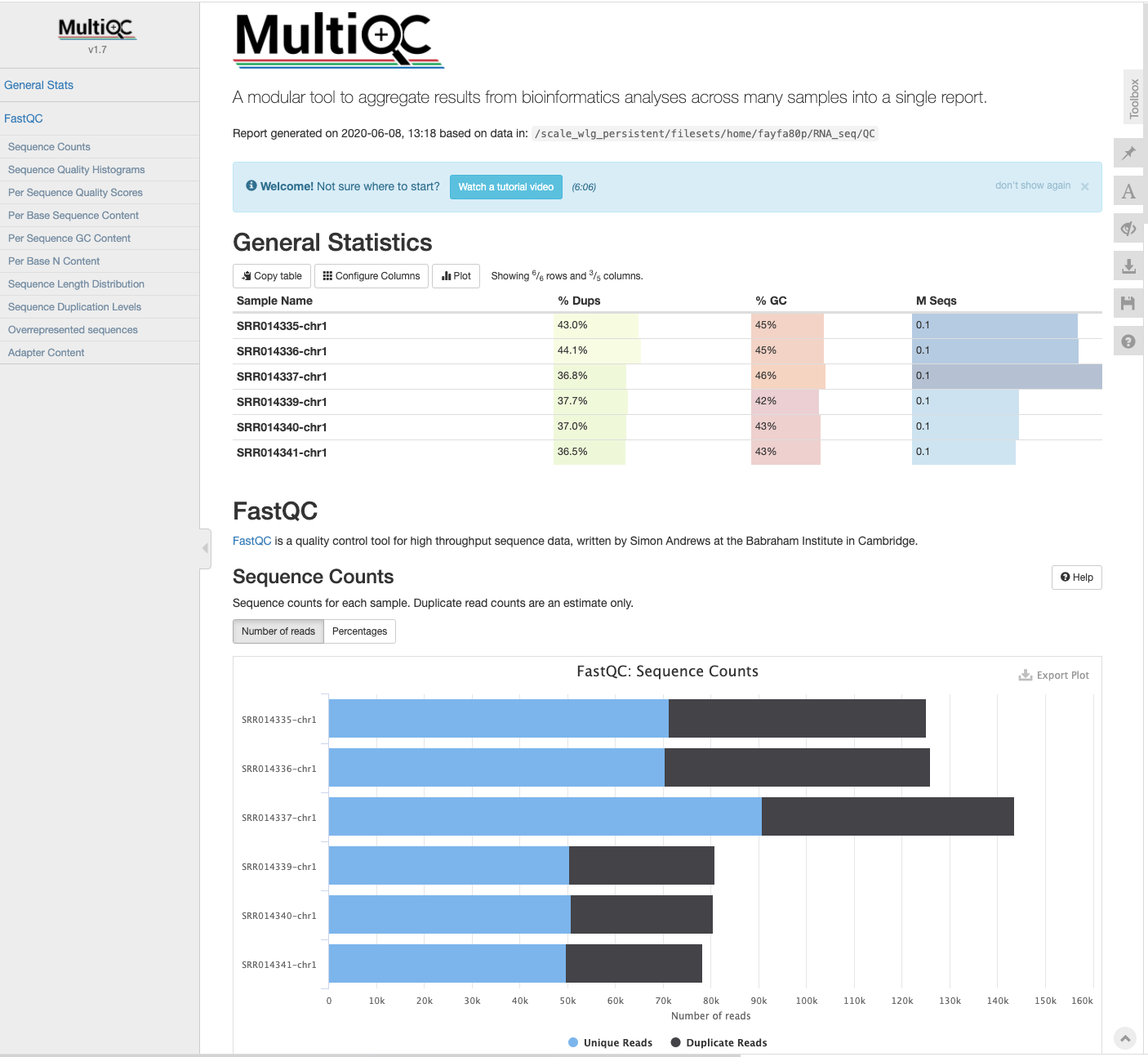
Use the MultiQC application to combine and view quality information
Several tools available to do quality assessemnt. For this workshop, we will use fastqc.
First, it is always good to verify where we are:
$ pwd
/home/[your_username]
# good I am ready to work

cd ~/obss_2021/
# copy the needed data into your directory
cp -r /nesi/projects/nesi02659/obss_2021/Resources/RNA_seq/ .
Checking to make sure we have the Raw files for the workshop.
$ ls
edna gbs genomic_dna intro_bash intro_r RNA_seq . ..
Creating a directory where to store the QC data:
$ cd RNA_seq
$ ls
Genome  Raw  rsmodules.sh  yeast_counts_all_chr.txt
$ mkdir QC
Since we are working on the NeSI HPC, we need to search and load the package before we start using it.
Search
$ module spider fastqc
and then load
$ module purge
$ module load FastQC/0.11.9
hint : there is a file named rsmodules.sh which is a shell script to load the required modules at once. Running
source ~/RNA_seq/rsmodules.shcommand will excute it.
Now we can start the quality control:
$ fastqc -o QC/ Raw/*
You will see an automatically updating output message telling you the progress of the analysis. It will start like this:
Started analysis of SRR014335-chr1.fastq
Approx 5% complete for SRR014335-chr1.fastq
Approx 10% complete for SRR014335-chr1.fastq
Approx 15% complete for SRR014335-chr1.fastq
Approx 20% complete for SRR014335-chr1.fastq
Approx 25% complete for SRR014335-chr1.fastq
Approx 30% complete for SRR014335-chr1.fastq
Approx 35% complete for SRR014335-chr1.fastq
The FastQC program has created several new files within our RNA_seq/QC/ directory.
$ ls QC
SRR014335-chr1_fastqc.html  SRR014336-chr1_fastqc.zip   SRR014339-chr1_fastqc.html  SRR014340-chr1_fastqc.zip
SRR014335-chr1_fastqc.zip   SRR014337-chr1_fastqc.html  SRR014339-chr1_fastqc.zip   SRR014341-chr1_fastqc.html
SRR014336-chr1_fastqc.html  SRR014337-chr1_fastqc.zip   SRR014340-chr1_fastqc.html  SRR014341-chr1_fastqc.zip
Viewing the FastQC results
If we were working on our local computers, we’d be able to look at each of these HTML files by opening them in a web browser.
However, these files are currently sitting on our remote NeSI HPC, where our local computer can’t see them. And, since we are only logging into NeSI via the command line - it doesn’t have any web browser setup to display these files either.
So the easiest way to look at these webpage summary reports will be to transfer them to our local computers (i.e. your laptop).
To transfer a file from a remote server to our own machines, we will use scp.
First we will make a new directory on our computer to store the HTML files we’re transferring. Let’s put it on our desktop for now. Open a new tab in your terminal program (you can use the pull down menu at the top of your screen or the Cmd+t keyboard shortcut) and type:
$ mkdir -p ~/Desktop/fastqc_html
$ scp -r [Your_UserName]p@login.mahuika.nesi.org.nz:~/obss_2021/RNA_seq/QC/ ~/Desktop/fastqc_html
Working with the FastQC text output
Now that we’ve looked at our HTML reports to get a feel for the data, let’s look more closely at the other output files. Go back to the tab in your terminal program that is connected to NeSI and make sure you’re in our results subdirectory.
$ cd /home/fayfa80p/obss_2021/RNA_seq/QC

$ ls
SRR014335-chr1_fastqc.html  SRR014336-chr1_fastqc.zip   SRR014339-chr1_fastqc.html  SRR014340-chr1_fastqc.zip
SRR014335-chr1_fastqc.zip   SRR014337-chr1_fastqc.html  SRR014339-chr1_fastqc.zip   SRR014341-chr1_fastqc.html
SRR014336-chr1_fastqc.html  SRR014337-chr1_fastqc.zip   SRR014340-chr1_fastqc.html  SRR014341-chr1_fastqc.zip
Let’s unzip the files to look at the FastQC text file outputs.
$ for filename in *.zip
> do
> unzip $filename
> done
Inside each unzipped folder, there is a summary text which shows results of the statistical tests done by FastQC
$ ls SRR014335-chr1_fastqc
fastqc_data.txt fastqc.fo fastqc_report.html Icons/ Images/ summary.txt
Use less to preview the summary.txt file
$ less SRR014335-chr1_fastqc/summary.txt
We can make a record of the results we obtained for all our samples by concatenating all of our summary.txt files into a single file using the cat command. We’ll call this fastqc_summaries.txt.
$ cat */summary.txt > ~/obss_2021/RNA_seq/QC/fastqc_summaries.txt
- Have a look at the fastqc_summaries.txt and search for any of the samples that have failed the QC statistical tests.
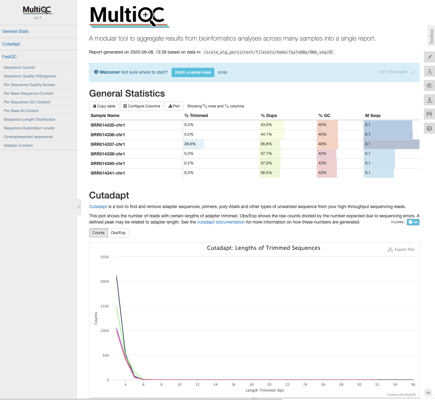
MultiQC - multi-sample analysis
- The FastQC analysis is applied to each sample separately, and produces a report for each.
- The application MultiQC provides a way to combine multiple sets of results (i.e., from MANY different software packages) across multipel samples.
- To generate
multqcresults, run the following command in the directory with the output files you want to summarise (e.g., fastqc reports generated above):
$ module load MultiQC/1.9-gimkl-2020a-Python-3.8.2
$ cd ~/obss_2021/RNA_seq/
$ mkdir MultiQC
$ cd MultiQC
$ cp ../QC/* ./
$ multiqc .
$ ls -F
multiqc_data/ multiqc_report.html
The html report shows the MultiQC summary
Key Points
Quality assessmet is a key initial step in the analysis of RNA-seq data
The FastQC and MultiQC applications are useful tools for quality assessent of RNA-seq data.
Trimming and Filtering reads
Overview
Teaching: 30 min
Exercises: 0 minQuestions
What steps are required for basic data cleaning in RNA-seq studies?
Objectives
Understand the various data cleaning steps for RNA-seq data.
Learn how to perfrorm adapter removal and quality trimming.
Cleaning Reads
In the previous section, we took a high-level look at the quality of each of our samples using FastQC. We visualized per-base quality graphs showing the distribution of read quality at each base across all reads in a sample and extracted information about which samples fail which quality checks. Some of our samples failed quite a few quality metrics used by FastQC. This doesn’t mean, though, that our samples should be thrown out! It’s very common to have some quality metrics fail, and this may or may not be a problem for your downstream application.
Adapter removal
- “Adapters” are short DNA sequences that are added to each read as part of the sequencing process (we won’t get into “why” here).
- These are removed as part of the data generation steps that occur during the sequencing run, but sometimes there is still a non-trivial amount of adapter sequence present in the FASTQ files.
- Since the sequence is not part of the target genome (i.e., the genome if the species from which teh samples were derived) then we need to remove it to prevent it affecting the downstream analysis.
- The FastQC application get detection adapter contamination in samples.
We will use a program called CutAdapt to filter poor quality reads and trim poor quality bases from our samples.
How to act on fastq after QC.
We can do several trimming:
- on quality using Phred score. What will be the Phred score?
- on the sequences, if they contain adaptor sequences.
To do so, we can use on tools: The cutadapt application is often used to remove adapter sequence from FASTQ files.
- The following syntax will remove the adapter sequence AACCGGTT from the file SRR014335-chr1.fastq, create a new file called SRR014335-chr1_trimmed.fastq, and write a summary to the log file SRR014335-chr1.log:
$ pwd
/home/[Your_Username]/obss_2021/RNA_seq

$ mkdir Trimmed

$ module load cutadapt/2.10-gimkl-2020a-Python-3.8.2

$ cutadapt -q 20 -a AACCGGTT -o Trimmed/SRR014335-chr1_cutadapt.fastq Raw/SRR014335-chr1.fastq > Trimmed/SRR014335-chr1.log
We can have a look at the log file to see what cutadapt has done.
$ less Trimmed/SRR014335-chr1.log
Now we should trim all samples.
$ cd Raw

$ ls
SRR014335-chr1.fastq SRR014336-chr1.fastq SRR014337-chr1.fastq SRR014339-chr1.fastq SRR014340-chr1.fastq SRR014341-chr1.fastq
$ for filename in *.fastq
> do base=$(basename ${filename} .fastq)
> cutadapt -q 20 -a AACCGGTT -o ../Trimmed/${base}.trimmed.fastq ${filename} > ../Trimmed/${base}.log
> done
MultiQC: cutadapt log files
- If the log files from
cutadaptare added to the directory containing the FastQC output, this information will also be incorporated into the MultiQC report the next time it is run.
$ cd ../MultiQC

$ cp ../Trimmed/*log .

$ multiqc .
Key Points
Adapter removal and trimming (optional) are important steps in processign RNA-seq data.
Map and count reads
Overview
Teaching: 45 min
Exercises: 0 minQuestions
How do we turn fastq data into read counts?
Objectives
Align reads to reference genome.
Assess read mapping for each sample.
Generate per-sample count data for each genomic feature (e.g., genes, exons etc) that you are interested in.
Alignment to a reference genome
RNA-seq generate gene expression information by quantifying the number of transcripts (per gene) in a sample. This is acompished by counting the number of transcripts that have been sequenced - the more active a gene is, the more transcripts will be in a sample, and the more reads will be generated from that transcript.
For RNA-seq, we need to align or map each read back to the genome, to see which gene produced it.
- Highly expressed genes will generate lots of transcripts, so there will be lots of reads that map back to the position of that transcript in the genome.
- The per-gene data we work with in an RNA-seq experiment are counts: the number of reads from each sample that originated from that gene.
Preparation of the genome
To be able to map (align) sequencing reads on the genome, the genome needs to be indexed first. In this workshop we will use HISAT2. Note for speed reason, the reads will be aligned on the chr5 of the mouse genome.
$ cd /home/[Your_Username]/obss_2021/RNA_seq/Genome

#to list what is in your directory:
$ ls /home/[Your_Username]/obss_2021/RNA_seq/Genome
Saccharomyces_cerevisiae.R64-1-1.99.gtf Saccharomyces_cerevisiae.R64-1-1.dna.toplevel.fa
$ module load HISAT2/2.2.0-gimkl-2020a

# index file:
$ hisat2-build -p 4 -f Saccharomyces_cerevisiae.R64-1-1.dna.toplevel.fa Saccharomyces_cerevisiae.R64-1-1.dna.toplevel

#list what is in the directory:
$ ls /home/[Your_Username]/obss_2021/RNA_seq/Genome
Saccharomyces_cerevisiae.R64-1-1.99.gtf              Saccharomyces_cerevisiae.R64-1-1.dna.toplevel.4.ht2  Saccharomyces_cerevisiae.R64-1-1.dna.toplevel.8.ht2
Saccharomyces_cerevisiae.R64-1-1.dna.toplevel.1.ht2  Saccharomyces_cerevisiae.R64-1-1.dna.toplevel.5.ht2  Saccharomyces_cerevisiae.R64-1-1.dna.toplevel.fa
Saccharomyces_cerevisiae.R64-1-1.dna.toplevel.2.ht2  Saccharomyces_cerevisiae.R64-1-1.dna.toplevel.6.ht2
Saccharomyces_cerevisiae.R64-1-1.dna.toplevel.3.ht2  Saccharomyces_cerevisiae.R64-1-1.dna.toplevel.7.ht2
Option info:
- -p number of threads
- -f fasta file
How many files were created during the indexing process?
Alignment on the genome
Now that the genome is prepared. Sequencing reads can be aligned.
Information required:
- Where the sequence information is stored (e.g. fastq files …) ?
- What kind of sequencing: Single End or Paired end ?
- Where are stored the indexes and the genome?
-
Where will the mapping files be stored?
- Now, lets move one folder up (into the RNA_seq folder):
$ cd ..

$ ls
Genome QC Raw Trimmed
Let’s map one of our sample to the genome
$ hisat2 -x Genome/Saccharomyces_cerevisiae.R64-1-1.dna.toplevel -U Raw/SRR014335-chr1.fastq -S SRR014335.sam
125090 reads; of these:
  125090 (100.00%) were unpaired; of these:
    20537 (16.42%) aligned 0 times
    85066 (68.00%) aligned exactly 1 time
    19487 (15.58%) aligned >1 times
83.58% overall alignment rate
Now we need to align all the rest of the samples.
$ pwd
/home/[Your_Username]/obss_2021/RNA_seq/
$ mkdir Mapping

$ ls
Genome Mapping QC Raw SRR014335.sam Trimmed
let’s use a for loop to process our samples:
$ cd Trimmed

$ ls
SRR014335-chr1.fastq SRR014336-chr1.fastq SRR014337-chr1.fastq SRR014339-chr1.fastq SRR014340-chr1.fastq SRR014341-chr1.fastq
$ for filename in *.trimmed.fastq
> do
> base=$(basename ${filename} .trimmed.fastq)
> hisat2 -p 4 -x ../Genome/Saccharomyces_cerevisiae.R64-1-1.dna.toplevel -U $filename -S ../Mapping/${base}.sam --summary-file ../Mapping/${base}_summary.txt
> done
Now we can explore our SAM files.
$ cd ../Mapping

$ ls
SRR014335-chr1.sam          SRR014336-chr1_summary.txt  SRR014339-chr1.sam          SRR014340-chr1_summary.txt
SRR014335-chr1_summary.txt  SRR014337-chr1.sam          SRR014339-chr1_summary.txt  SRR014341-chr1.sam
SRR014336-chr1.sam          SRR014337-chr1_summary.txt  SRR014340-chr1.sam          SRR014341-chr1_summary.txt
Converting SAM files to BAM files
The SAM file, is a tab-delimited text file that contains information for each individual read and its alignment to the genome. While we do not have time to go into detail about the features of the SAM format, the paper by Heng Li et al. provides a lot more detail on the specification.
The compressed binary version of SAM is called a BAM file. We use this version to reduce size and to allow for indexing, which enables efficient random access of the data contained within the file.
A quick look into the sam file
$ less SRR014335-chr1.sam
The file begins with a header, which is optional. The header is used to describe the source of data, reference sequence, method of alignment, etc., this will change depending on the aligner being used. Following the header is the alignment section. Each line that follows corresponds to alignment information for a single read. Each alignment line has 11 mandatory fields for essential mapping information and a variable number of other fields for aligner specific information. An example entry from a SAM file is displayed below with the different fields highlighted.
We will convert the SAM file to BAM format using the samtools program with the view command and tell this command that the input is in SAM format (-S) and to output BAM format (-b):
$ module load SAMtools/1.10-GCC-9.2.0

$ for filename in *.sam
> do
> base=$(basename ${filename} .sam)
> samtools view -S -b ${filename} -o ${base}.bam
> done

$ ls
SRR014335-chr1.bam  SRR014336-chr1.bam  SRR014337-chr1.bam  SRR014339-chr1.bam  SRR014340-chr1.bam  SRR014341-chr1.bam
SRR014335-chr1.sam  SRR014336-chr1.sam  SRR014337-chr1.sam  SRR014339-chr1.sam  SRR014340-chr1.sam  SRR014341-chr1.sam
Sorting BAM files
Next we sort the BAM file using the sort command from samtools. -o tells the command where to write the output.
$ for filename in *.bam
> do
> base=$(basename ${filename} .bam)
> samtools sort -o ${base}_sorted.bam ${filename}
> done
SAM/BAM files can be sorted in multiple ways, e.g. by location of alignment on the chromosome, by read name, etc. It is important to be aware that different alignment tools will output differently sorted SAM/BAM, and different downstream tools require differently sorted alignment files as input.
You can use samtools to learn more about the bam file as well.
Some stats on your mapping:
$ samtools flagstat SRR014335-chr1_sorted.bam
156984 + 0 in total (QC-passed reads + QC-failed reads)
31894 + 0 secondary
0 + 0 supplementary
0 + 0 duplicates
136447 + 0 mapped (86.92% : N/A)
0 + 0 paired in sequencing
0 + 0 read1
0 + 0 read2
0 + 0 properly paired (N/A : N/A)
0 + 0 with itself and mate mapped
0 + 0 singletons (N/A : N/A)
0 + 0 with mate mapped to a different chr
0 + 0 with mate mapped to a different chr (mapQ>=5)
MultiQC: HISAT2 output
- The HISAT2 output data can also be incorporated into the MultiQC report the next time it is run.
 $ cd ~/obss_2021/RNA_seq/MultiQC

 $ cp ../Mapping/*summary* ./

 $ multiqc .
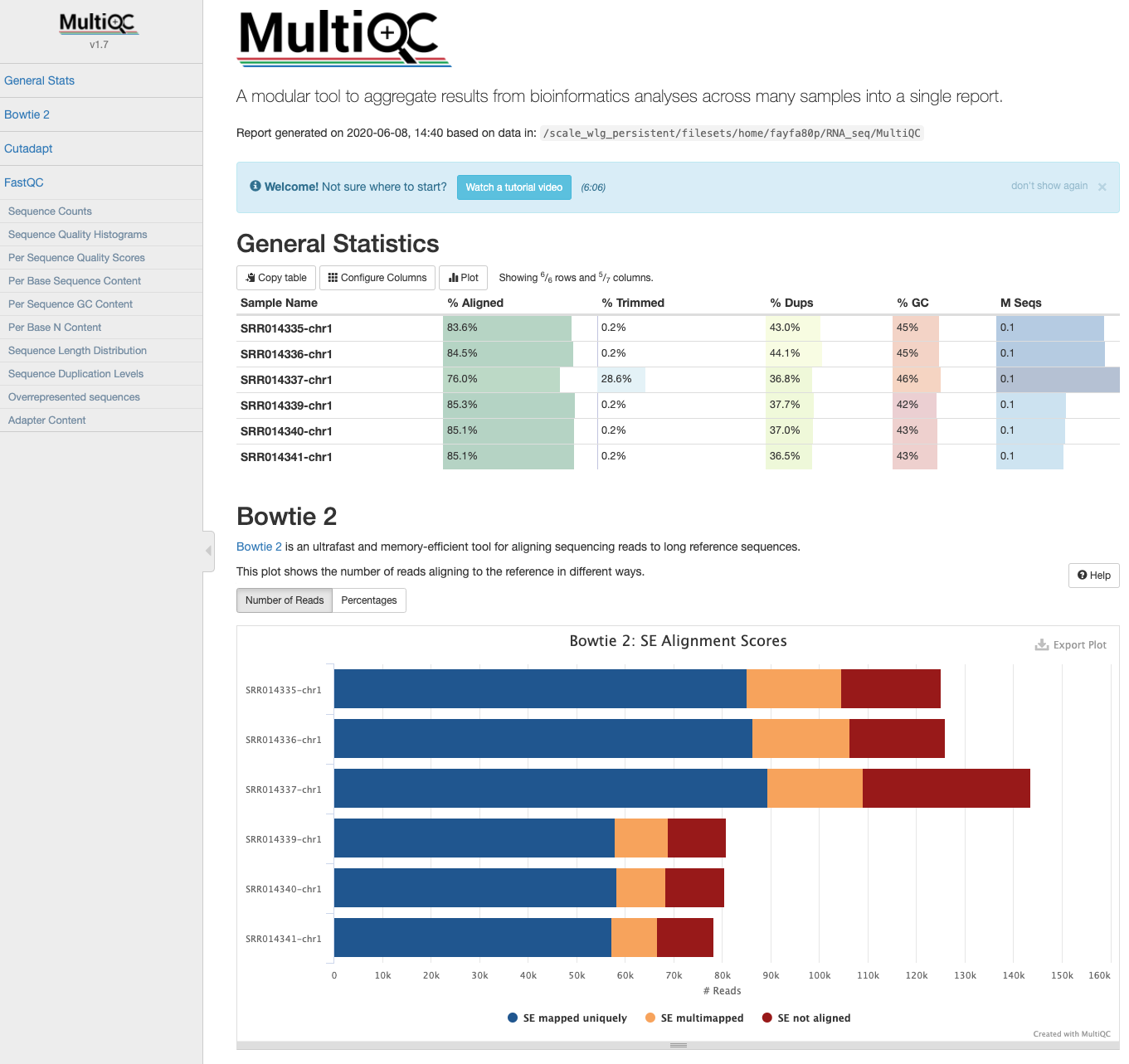
Please note: running HISAT2 with either option --summary-file or older versions (< v2.1.0) gives log output identical to Bowtie2. These logs are indistinguishable and summary statistics will appear in MultiQC reports labelled as Bowtie2.
Read Summarization
Sequencing reads often need to be assigned to genomic features of interest after they are mapped to the reference genome. This process is often called read summarization or read quantification. Read summarization is required by a number of downstream analyses such as gene expression analysis and histone modification analysis. The output of read summarization is a count table, in which the number of reads assigned to each feature in each library is recorded.
Counting
- We need to do some counting!
- Want to generate count data for each gene (actually each exon) - how many reads mapped to each exon in the genome, from each of our samples?
- Once we have that information, we can start thinking about how to determine which genes were differentially expressed in our study.
Subread and FeatureCounts
- The featureCounts tool from the Subread package can be used to count how many reads aligned to each genome feature (exon).
- Need to specify the annotation informatyion (.gtf file) You can process all the samples at once:
$ module load Subread

$ pwd
/home/[Your_Username]/obss_2021/RNA_seq

$ mkdir Counts

$ cd Counts

$ featureCounts -a ../Genome/Saccharomyces_cerevisiae.R64-1-1.99.gtf -o ./yeast_counts.txt -T 2 -t exon -g gene_id ../Mapping/*sorted.bam
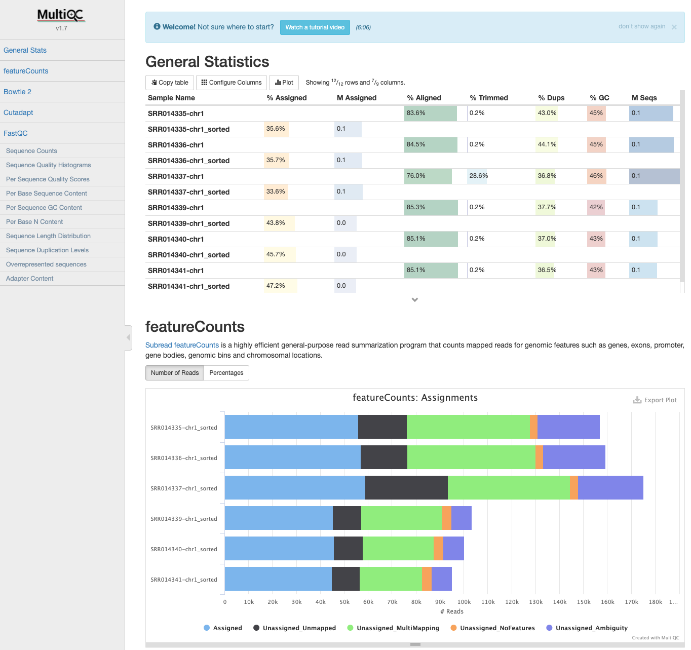
MultiQC: featureCounts output
- If the samples are processed individually, the output data can be incorporated into the MultiQC report the next time it is run.
$ cd ../MultiQC

$ cp ../Counts/* .

$ multiqc .
Since we now have all the count data in one file, we need to transfer it to our local computers so we could start working on RStudio to get differentially expressed genes.
- And the code to do it is below, however for this workshop, we are going to use a different file (yeast_counts_all_chr.txt) that you can download from section 4. Differential_Expression. This file has all the data for all the chromosomes.
#In a new terminal that you can access you computer files, cd to the directory you want to save the counts file.

$ scp fayfa80p@login.mahuika.nesi.org.nz:/home/fayfa80p/RNA_seq/Counts/yeast_counts_all_chr.txt ./
Download with Jupyter
An alternative is to navigate to the directory
~/obss_2021/RNA_seq/Counts/in the navigation panel of Jupyter then right-click onyeast_counts_all_chr.txtand select “Download”
Key Points
Alignment and feature counting are used to generate read counts for each genomic feature (e.g., genes) of interest, per sample.
The count data can then be used for stataistical analysis (e.g., to identify differentially expressed genes).
Differential Expression
Overview
Teaching: 75 min
Exercises: 0 minQuestions
How can we identify genes which exhibit changes in expresion between experimental conditions?
Objectives
Understand pre-processing steps required for standarising count data.
Use count data and the limma package to perform normalisation and identify differentially expressed genes.
Understand need for multiple comparisons correction, and be able to apply FWER and FDR correction methods.
Explore alternative methods (egdeR and DESeq2) for identifying differentially expressed genes.
RNA-seq: overview
Recap
- In the last section we worked through the process of quality assessment and alignment for RNA-seq data
- This typically takes place on the command line, but can also be done from within R.
- The end result was the generation of count data (counts of reads aligned to each gene, per sample) using the FeatureCounts command from Subread/Rsubread.
- Now that we’ve got count data in R, we can begin our differential expression analysis.
Data set reminder
- Data obtained from yeast RNA-seq experiment, Lee et al 2008
- Wild-type versus RNA degradation mutants
- Six samples (3 WT / 3 MT)
- NOTE: since we are dealing with an RNA degradation mutant yeast strain, we will see MAJOR transcriptomic differences between the wild-type and mutant groups (usually the differences you observe in a typical RNA-seq study wouldn’t be this extreme).
Getting organised
NOTE: skip to the next section (“Count Data”) if you are working within Jupyter on NeSI
Create an RStudio project
One of the first benefits we will take advantage of in RStudio is something called an RStudio Project. An RStudio project allows you to more easily:
- Save data, files, variables, packages, etc. related to a specific analysis project
- Restart work where you left off
- Collaborate, especially if you are using version control such as git.
To create a project:
- Open RStudio and go to the File menu, and click New Project.
- In the window that opens select Existing Project, and browse to the RNA_seq folder.
- Finally, click Create Project.
Save source from untitled to
yeast_data.Rand continue saving regularly as you work.
Lecture notes
In addition to the code below, we’ll also be going through some lecture notes that explain the various concepts being covered in this part of the workshop.
Lecture notes (PDF): Differential Expression
Count data
Note: I have now aligned the data for ALL CHROMOSOMES and generated counts, so we are working with data from all 7127 genes.
Let’s look at our data set and perform some basic checks before we do a differential expression analysis.
Working directory in Jupyter
Before launching your R notebook in Jupyter, navigate to
~/obss_2021/RNA_seq/in the navigation panel. Ensure your working directory by usinggetwd()and if it isn’t~/obss_2021/RNA_seq/, set it withsetwd('~/obss_2021/RNA_seq').
library(dplyr)
fcData = read.table('yeast_counts_all_chr.txt', sep='\t', header=TRUE)
fcData %>% head()
    ##      Geneid Chr Start   End Strand Length ...STAR.SRR014335.Aligned.out.sam
    ## 1   YDL248W  IV  1802  2953      +   1152                                52
    ## 2 YDL247W-A  IV  3762  3836      +     75                                 0
    ## 3   YDL247W  IV  5985  7814      +   1830                                 2
    ## 4   YDL246C  IV  8683  9756      -   1074                                 0
    ## 5   YDL245C  IV 11657 13360      -   1704                                 0
    ## 6   YDL244W  IV 16204 17226      +   1023                                 6
    ##   ...STAR.SRR014336.Aligned.out.sam ...STAR.SRR014337.Aligned.out.sam
    ## 1                                46                                36
    ## 2                                 0                                 0
    ## 3                                 4                                 2
    ## 4                                 0                                 1
    ## 5                                 3                                 0
    ## 6                                 6                                 5
    ##   ...STAR.SRR014339.Aligned.out.sam ...STAR.SRR014340.Aligned.out.sam
    ## 1                                65                                70
    ## 2                                 0                                 1
    ## 3                                 6                                 8
    ## 4                                 1                                 2
    ## 5                                 5                                 7
    ## 6                                20                                30
    ##   ...STAR.SRR014341.Aligned.out.sam
    ## 1                                78
    ## 2                                 0
    ## 3                                 5
    ## 4                                 0
    ## 5                                 4
    ## 6                                19
Check dimensions:
dim(fcData)
## [1] 7127 12
names(fcData)
    ##  [1] "Geneid"                            "Chr"
    ##  [3] "Start"                             "End"
    ##  [5] "Strand"                            "Length"
    ##  [7] "...STAR.SRR014335.Aligned.out.sam" "...STAR.SRR014336.Aligned.out.sam"
    ##  [9] "...STAR.SRR014337.Aligned.out.sam" "...STAR.SRR014339.Aligned.out.sam"
    ## [11] "...STAR.SRR014340.Aligned.out.sam" "...STAR.SRR014341.Aligned.out.sam"
Rename data columns to reflect group membership
names(fcData)[7:12] = c("WT1", "WT2", "WT3", "MT1", "MT2", "MT3")

fcData %>% head()
    ##      Geneid Chr Start   End Strand Length WT1 WT2 WT3 MT1 MT2 MT3
    ## 1   YDL248W  IV  1802  2953      +   1152  52  46  36  65  70  78
    ## 2 YDL247W-A  IV  3762  3836      +     75   0   0   0   0   1   0
    ## 3   YDL247W  IV  5985  7814      +   1830   2   4   2   6   8   5
    ## 4   YDL246C  IV  8683  9756      -   1074   0   0   1   1   2   0
    ## 5   YDL245C  IV 11657 13360      -   1704   0   3   0   5   7   4
    ## 6   YDL244W  IV 16204 17226      +   1023   6   6   5  20  30  19
Extract count data
- Remove annotation columns
- Add row names
counts = fcData[, 7:12]
rownames(counts) = fcData$Geneid
counts %>% head()
    ##           WT1 WT2 WT3 MT1 MT2 MT3
    ## YDL248W    52  46  36  65  70  78
    ## YDL247W-A   0   0   0   0   1   0
    ## YDL247W     2   4   2   6   8   5
    ## YDL246C     0   0   1   1   2   0
    ## YDL245C     0   3   0   5   7   4
    ## YDL244W     6   6   5  20  30  19
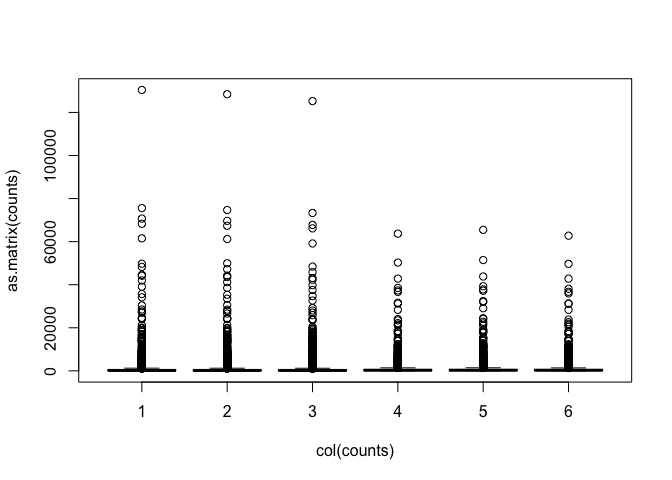
Visualising the data
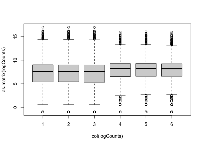
Data are highly skewed (suggests that logging might be useful):
boxplot(as.matrix(counts) ~ col(counts))
Some genes have zero counts:
colSums(counts==0)
    ## WT1 WT2 WT3 MT1 MT2 MT3
    ## 562 563 573 437 425 435
Log transformation (add 0.5 to avoid log(0) issues):
logCounts = log2(as.matrix(counts)+ 0.5)
Now we can see the per-sample distributions more clearly:
boxplot(as.matrix(logCounts) ~ col(logCounts))
Density plots are also a good way to visualise the data:
lineColour <- c("blue", "blue", "blue", "red", "red", "red")
lineColour
## [1] "blue" "blue" "blue" "red" "red" "red"
plot(density(logCounts[,1]), ylim=c(0,0.3), col=lineColour[1])
for(i in 2:ncol(logCounts)) lines(density(logCounts[,i]), col=lineColour[i])
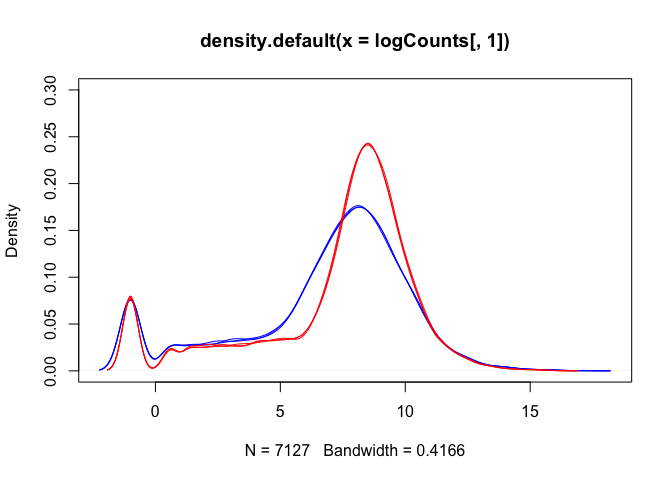
The boxplots and density plots show clear differences between the sample groups - are these biological, or experimental artifacts? (often we don’t know).
Remember: the wild-type and mutant yeast strains are VERY different. You wouldn’t normally see this amount of difference in the distributions between the groups.
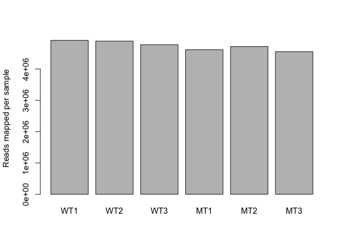
Read counts per sample
Normalisation process (slightly different for each analysis method) takes “library size” (number of reads generated for each sample) into account.
- A good blog about normalization: Link
colSums(counts)
    ##     WT1     WT2     WT3     MT1     MT2     MT3
    ## 4915975 4892227 4778158 4618409 4719413 4554283
Visualise via bar plot
colSums(counts) %>% barplot(., ylab="Reads mapped per sample")
Now we are ready for differential expression analysis
Detecting differential expression:
We are going to identify genes that are differential expressed using 3 different packages (time allowing) and compare the results.
But first, lets take a brief aside, and talk about the process of detecting genes that have undergone a statistically significance change in expression between the two groups.
Limma
- Limma can be used for analysis, by transforming the RNA-seq count data in an appropriate way (log-scale normality-based assumption rather than Negative Binomial for count data)
- Use data transformation and log to satisfy normality assumptions (CPM = Counts per Million).
library(limma)
library(edgeR)

dge <- DGEList(counts=counts)
dge <- calcNormFactors(dge)
logCPM <- cpm(dge, log=TRUE, prior.count=3)

options(width=100)
head(logCPM, 3)
    ##                  WT1        WT2        WT3        MT1        MT2        MT3
    ## YDL248W    3.7199528  3.5561232  3.2538405  3.6446399  3.7156488  3.9155366
    ## YDL247W-A -0.6765789 -0.6765789 -0.6765789 -0.6765789 -0.3140297 -0.6765789
    ## YDL247W    0.1484688  0.6727144  0.1645731  0.7843936  1.0395626  0.6349276
Aside: RPKM
We can use R to generate RPKM values (or FPKM if using paired-end reads):
- Need gene length information to do this
- Can get this from
goseqpackage (we’ll use this later for our pathway analysis)
library(goseq)
geneLengths = getlength(rownames(counts), "sacCer2","ensGene")
rpkmData <- rpkm(dge, geneLengths)
rpkmData %>% round(., 2) %>% head()
    ##             WT1  WT2  WT3   MT1   MT2   MT3
    ## YDL248W   10.89 9.66 7.73 10.30 10.85 12.55
    ## YDL247W-A  0.00 0.00 0.00  0.00  2.35  0.00
    ## YDL247W    0.26 0.53 0.27  0.60  0.78  0.51
    ## YDL246C    0.00 0.00 0.23  0.17  0.33  0.00
    ## YDL245C    0.00 0.43 0.00  0.54  0.73  0.44
    ## YDL244W    1.41 1.42 1.21  3.57  5.24  3.44
range(rpkmData, na.rm=TRUE)
## [1] 0.00 69786.58
Compare RPKM to logCPM
par(mfrow=c(2,3))
for(i in 1:ncol(rpkmData)){
  plot(logCPM[,i], log2(rpkmData[,i]), pch='.',
       xlab="logCPM", ylab="RPKM", main=colnames(logCPM)[i])
}
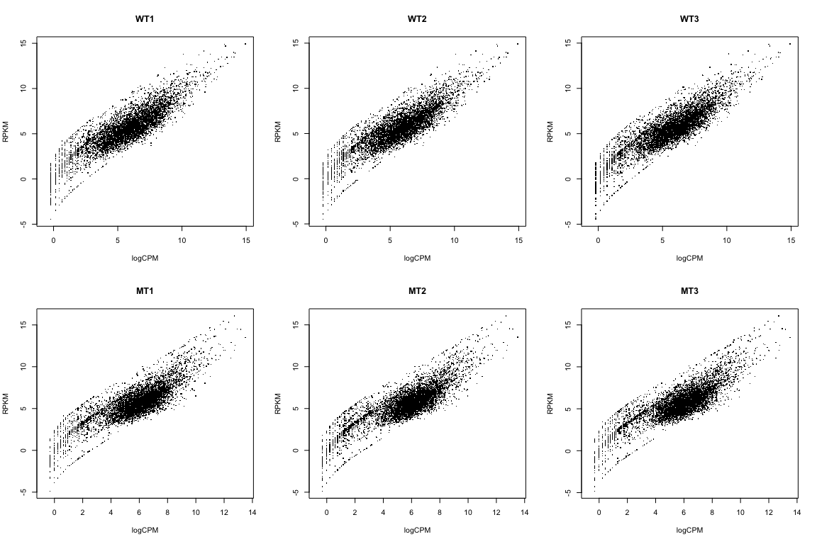
We’re NOT going to use RPKM data here. I just wanted to show you how to calculate it, and how it relates to the logCPM data
Back to the analysis… (using logCPM)
What if we just did a t-test?
## The beeswarm package is great for making jittered dot plots
library(beeswarm)

# Specify "conditions" (groups: WT and MT)
conds <- c("WT","WT","WT","MT","MT","MT")

## Perform t-test for "gene number 6" (because I like that one...)
t.test(logCPM[6,] ~ conds)
    ##
    ##  Welch Two Sample t-test
    ##
    ## data:  logCPM[6, ] by conds
    ## t = 7.0124, df = 2.3726, p-value = 0.01228
    ## alternative hypothesis: true difference in means is not equal to 0
    ## 95 percent confidence interval:
    ##  0.5840587 1.9006761
    ## sample estimates:
    ## mean in group MT mean in group WT
    ##         2.244310         1.001943
beeswarm(logCPM[6,] ~ conds, pch=16, ylab="Expression (logCPM)", xlab="Group",
         main=paste0(rownames(logCPM)[6], ": MT vs WT"))
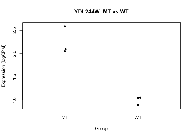
- we basically want to do this sort of analysis, for every gene
- we’ll use a slightly more sophisticated approach though
However, before we get to statistical testing, we (might) first need to do a little bit more normalisation.
Limma: voom
- The “voom” function estimates relationship between the mean and the variance of the logCPM data, normalises the data, and creates “precision weights” for each observation that are incorporated into the limma analysis.
design <- model.matrix(~conds)
design
    ##   (Intercept) condsWT
    ## 1           1       1
    ## 2           1       1
    ## 3           1       1
    ## 4           1       0
    ## 5           1       0
    ## 6           1       0
    ## attr(,"assign")
    ## [1] 0 1
    ## attr(,"contrasts")
    ## attr(,"contrasts")$conds
    ## [1] "contr.treatment"
v <- voom(dge, design, plot=TRUE)
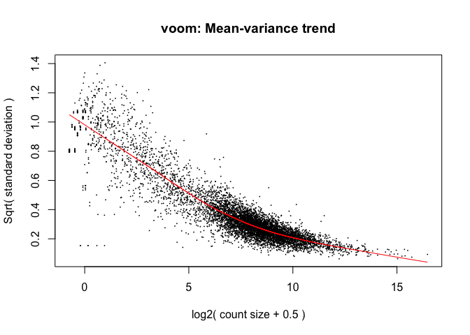
Voom: impact on samples
Mainly affects the low-end (low abundance genes)
par(mfrow=c(2,3))
for(i in 1:ncol(logCPM)){
  plot(logCPM[,i], v$E[,i], xlab="LogCPM",
       ylab="Voom",main=colnames(logCPM)[i])
  abline(0,1)
}

Hasn’t removed the differences between the groups
boxplot(v$E ~ col(v$E))

lineColour <- ifelse(conds=="MT", "red", "blue")
lineColour
## [1] "blue" "blue" "blue" "red" "red" "red"
plot(density(v$E[,1]), ylim=c(0,0.3), col=lineColour[1])
for(i in 2:ncol(logCPM)) lines(density(v$E[,i]), col=lineColour[i])

We can deal with this via “quantile normalisation”. Specify
normalize="quantile"
in the voom function.
q <- voom(dge, design, plot=TRUE, normalize="quantile")

Quantile normalisation forces all of the distributions to be the same.
- it is a strong assumption, and can have a major impact on the analysis
- potentially removing biological differences between groups.
par(mfrow=c(2,3))
for(i in 1:ncol(logCPM)){
  plot(logCPM[,i], q$E[,i], xlab="LogCPM",
       ylab="Voom (+quantile norm)",main=colnames(logCPM)[i])
  abline(0,1)
}

boxplot(q$E ~ col(q$E))

lineColour <- ifelse(conds=="MT", "red", "blue")
lineColour
## [1] "blue" "blue" "blue" "red" "red" "red"
plot(density(q$E[,1]), ylim=c(0,0.3), col=lineColour[1])
for(i in 2:ncol(logCPM)) lines(density(q$E[,i]), col=lineColour[i])

Note: we’re NOT going to use the quantile normalised data here, but I wanted to show you how that method works.
Statistical testing: fitting a linear model
The next step is to fit a linear model to the transformed count data.
The lmFit() command does this for each gene (all at once).
fit <- lmFit(v, design)
The eBayes() function then performs Emprical Bays shrinkage estimation
to adjust the variability estimates for each gene, and produce the
moderated t-statistics.
fit <- eBayes(fit)
We then summarize this information using the topTable() function,
which list the genes in order of the strength of statistical support for
differential expression (i.e., genes with lowest p-values are at the top
of the list):
tt <- topTable(fit, coef=ncol(design), n=nrow(counts))
head(tt)
##            logFC  AveExpr        t      P.Value    adj.P.Val        B
## YAL038W 2.313985 10.80214 319.5950 3.725452e-13 8.850433e-10 21.08951
## YOR161C 2.568389 10.80811 321.9628 3.574510e-13 8.850433e-10 21.08187
## YML128C 1.640664 11.40819 286.6167 6.857932e-13 9.775297e-10 20.84520
## YMR105C 2.772539  9.65092 331.8249 3.018547e-13 8.850433e-10 20.16815
## YHL021C 2.034496 10.17510 269.4034 9.702963e-13 1.152550e-09 20.07857
## YDR516C 2.085424 10.05426 260.8061 1.163655e-12 1.184767e-09 19.87217
Significant genes
Adjusted p-values less than 0.05:
sum(tt$adj.P.Val < 0.05)
## [1] 5140
Adjusted p-values less than 0.01:
sum(tt$adj.P.Val <= 0.01)
## [1] 4566
By default, limma uses FDR adjustment (but lets check):
sum(p.adjust(tt$P.Value, method="fdr") <= 0.01)
## [1] 4566
Volcano plots are a popular method for summarising the limma output:
volcanoplot(fit, coef=2)
abline(h=-log10(0.05))

Significantly DE genes:
sigGenes = which(tt$adj.P.Val <= 0.05)
length(sigGenes)
## [1] 5140
volcanoplot(fit, coef=2)
points(tt$logFC[sigGenes], -log10(tt$P.Value[sigGenes]), col='red', pch=16, cex=0.5)

Significantly DE genes above fold-change threshold:
sigGenes = which(tt$adj.P.Val <= 0.05 & (abs(tt$logFC) > log2(2)))
length(sigGenes)
## [1] 1891
volcanoplot(fit, coef=2)
points(tt$logFC[sigGenes], -log10(tt$P.Value[sigGenes]), col='red', pch=16, cex=0.5)

Get the rows of top table with significant adjusted p-values - we’ll save these for later to compare with the other methods.
limmaPadj <- tt[tt$adj.P.Val <= 0.01, ]
DESeq2
- The DESeq2 package uses the Negative Binomial distribution to model the count data from each sample.
- A statistical test based on the Negative Binomial distribution (via a generalized linear model, GLM) can be used to assess differential expression for each gene.
- Use of the Negative Binomial distribution attempts to accurately capture the variation that is observed for count data.
More information about DESeq2: article by Love et al, 2014
Set up “DESeq object” for analysis:
library(DESeq2)
dds <- DESeqDataSetFromMatrix(countData = as.matrix(counts),
                              colData = data.frame(conds=factor(conds)),
                              design = formula(~conds))
Can access the count data in teh dds object via the counts()
function:
counts(dds) %>% head()
##           WT1 WT2 WT3 MT1 MT2 MT3
## YDL248W    52  46  36  65  70  78
## YDL247W-A   0   0   0   0   1   0
## YDL247W     2   4   2   6   8   5
## YDL246C     0   0   1   1   2   0
## YDL245C     0   3   0   5   7   4
## YDL244W     6   6   5  20  30  19
Fit DESeq model to identify DE transcripts
dds <- DESeq(dds)
Take a look at the results table
res <- DESeq2::results(dds)
knitr::kable(res[1:6,])
| baseMean | log2FoldChange | lfcSE | stat | pvalue | padj | |
|---|---|---|---|---|---|---|
| YDL248W | 56.2230316 | -0.2339470 | 0.2278417 | -1.0267961 | 0.3045165 | 0.3663639 |
| YDL247W-A | 0.1397714 | -0.5255769 | 4.0804729 | -0.1288030 | 0.8975136 | 0.9173926 |
| YDL247W | 4.2428211 | -0.8100552 | 0.8332543 | -0.9721584 | 0.3309718 | 0.3948536 |
| YDL246C | 0.6182409 | -1.0326364 | 2.1560899 | -0.4789394 | 0.6319817 | 0.6915148 |
| YDL245C | 2.8486580 | -1.9781751 | 1.1758845 | -1.6822869 | 0.0925132 | 0.1230028 |
| YDL244W | 13.0883354 | -1.5823354 | 0.5128788 | -3.0852037 | 0.0020341 | 0.0032860 |
Summary of differential gene expression
summary(res)
##
## out of 6830 with nonzero total read count
## adjusted p-value < 0.1
## LFC > 0 (up)       : 2520, 37%
## LFC < 0 (down)     : 2521, 37%
## outliers [1]       : 0, 0%
## low counts [2]     : 0, 0%
## (mean count < 0)
## [1] see 'cooksCutoff' argument of ?results
## [2] see 'independentFiltering' argument of ?results
Note: p-value adjustment
- The “padj” column of the DESeq2 results (
res) contains adjusted p-values (FDR). - Can use the
p.adjustfunction to manually adjust the DESeq2 p-values if needed (e.g., to use Holm correction)
# Remove rows with NAs
res = na.omit(res)

# Get the rows of "res" with significant adjusted p-values
resPadj<-res[res$padj <= 0.05 , ]

# Get dimensions
dim(resPadj)
## [1] 4811 6
Number of adjusted p-values less than 0.05
sum(res$padj <= 0.05)
## [1] 4811
Check that this is the same using p.adjust with FDR correction
sum(p.adjust(res$pvalue, method="fdr") <= 0.05)
## [1] 4811
Number of Holm adjusted p-values less than 0.05
sum(p.adjust(res$pvalue, method="holm") <= 0.01)
## [1] 3429
Sort summary list by p-value and save the table as a CSV file that can be read in Excel (or any other spreadhseet program).
res <- res[order(res$padj),]

write.csv(as.data.frame(res),file='deseq2.csv')
edgeR
- The edgeR package also uses the negative binomial distribution to model the RNA-seq count data.
- Takes an empirical Bayes approach to the statistical analysis, in a
similar way to how the
limmapackage handles RNA-seq data.
Identify DEGs with edgeR’s “Exact” Method
Load edgeR package
library(edgeR)
Construct DGEList object
y <- DGEList(counts=counts, group=conds)
Calculate library size (counts per sample)
y <- calcNormFactors(y)
Estimate common dispersion (overall variability)
y <- estimateCommonDisp(y)
Estimate tagwise dispersion (per gene variability)
y <- estimateTagwiseDisp(y)
edgeR analysis and output
Compute exact test for the negative binomial distribution.
et <- exactTest(y)

knitr::kable(topTags(et, n=4)$table)
| logFC | logCPM | PValue | FDR | |
|---|---|---|---|---|
| YCR077C | 13.098599 | 6.629306 | 0 | 0 |
| snR71 | -9.870811 | 8.294459 | 0 | 0 |
| snR59 | -8.752555 | 10.105453 | 0 | 0 |
| snR53 | -8.503101 | 7.687908 | 0 | 0 |
Adjusted p-values
edge <- as.data.frame(topTags(et, n=nrow(counts)))
sum(edge$FDR <= 0.05)
## [1] 5242
sum(p.adjust(edge$PValue, method="fdr") <= 0.05)
## [1] 5242
Get the rows of “edge” with significant adjusted p-values
edgePadj <- edge[edge$FDR <= 0.05, ]
DESeq2 vs edgeR
Generate Venn diagram to compare DESeq2 and edgeR results.
There is fairly good overlap:
library(gplots)
setlist <- list(edgeRexact=rownames(edgePadj), DESeq2=rownames(resPadj))
venn(setlist)

Limma vs edgeR vs DESeq2
Again, fairly good overlap across the three methods we’ve looked at:
setlist <- list(edgeRexact=rownames(edgePadj),
                DESeq2=rownames(resPadj),
                LimmaVoom=rownames(limmaPadj))
venn(setlist)

Summary
- Once we’ve generated count data, there are a number of ways to
perform a differential expression analysis.
- DESeq2 and edgeR model the count data, and assume a Negative Binomial distribution
- Limma transforms (and logs) the data and assumes normality
- Here we’ve seen that these three approaches give quite similar results.
- The next step in a “standard” RNA-seq workflow is to perform “pathway analysis”.
Save limma topTable results for next session…
save(list='tt', file='topTable.RData')
Key Points
Statistical analysis is required to identify genes exhibiting altered expression between experimental conditions.
The limma processing pipeline is a fairly standard (and robust) way to do this.
DESeq2 and edgeR offer alternative methods for identifying differetially expressed genes.
Overrepresentation analysis (Gene Ontology)
Overview
Teaching: 60 min
Exercises: 0 minQuestions
How can we identify changes in biological mechanisms (e.g., pathways) in gene expression studies?
Objectives
Gain basic understanding of Gene Ontology.
Understand how over-representation analysis works for collections of genes.
Gain insight into the need for gene-length adjustment when performing over-representation analysis with RNA-seq data.
Use the GOseq methodology to identify gene-set changes based on Gene Ontology groups.
Lecture notes
In addition to the code below, we’ll also be going through some lecture notes that explain the various concepts being covered in this part of thw workshop.
Lecture notes (PDF): Annotation and Pathways
Overrepresentation analysis (Gene Ontology)
Over Representation Analysis (Boyle et al. 2004) is a widely used approach to determine whether known biological functions or processes are over-represented (= enriched) in an experimentally-derived gene list, e.g. a list of differentially expressed genes (DEGs).
- Can perform overrepresentation analysis online (e.g., Enrichr, GeneSetDB, PantherDB), and also in R.
- The basic principles are to:
- identify a collection of differentially expressed genes
- test to see if genes that are members of specific gene sets (e.g., Reactome pathways, Gene Ontology categories) are differentially expressed more often than would be expected by chance.
Some caveats for RNA-seq data
- The gene-set analysis methods are applicable to transcriptomic data from both microarrays and RNA-seq.
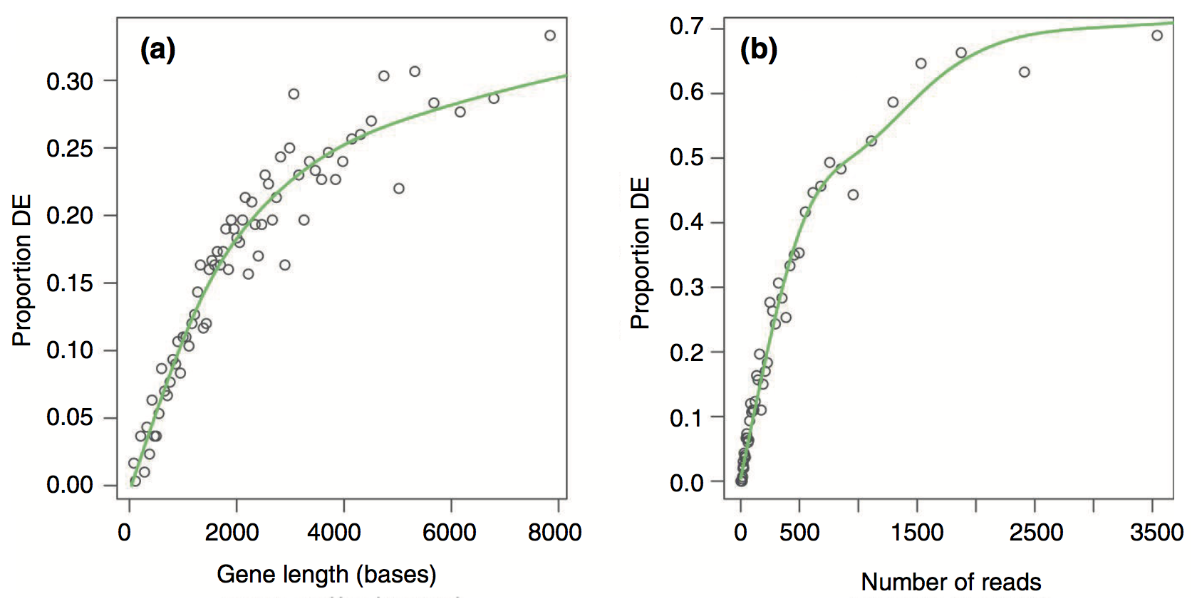
- One caveat, however, is that the results need to take gene length into account.
- RNA-seq tends to produce higher expression levels (i.e., greater counts) for longer genes: a longer transcript implies more aligned fragments, and thus higher counts. This also gives these genes a great chance of being statistically differentially expressed.
- Some gene sets (pathways, GO terms) tend to involve families of long genes: if long genes have a great chance of being detected as differentially expressed, then gene sets consisting of long genes will have a great chance of appeared to be enriched in the analysis.
GOseq
- The GOseq methodology (Young et al., 2010) overcomes this issue by allowing the over-representation analysis to be adjusted for gene length.
- modification to hypergeometric sampling probability
- exact method (resampling) and an approximation-based method
- More recent publications have also applied this gene-length correction to GSEA-based methods.
- Still not widely understood to be an issue when performing RNA-seq pathway analysis, but REALLY important to take into account.
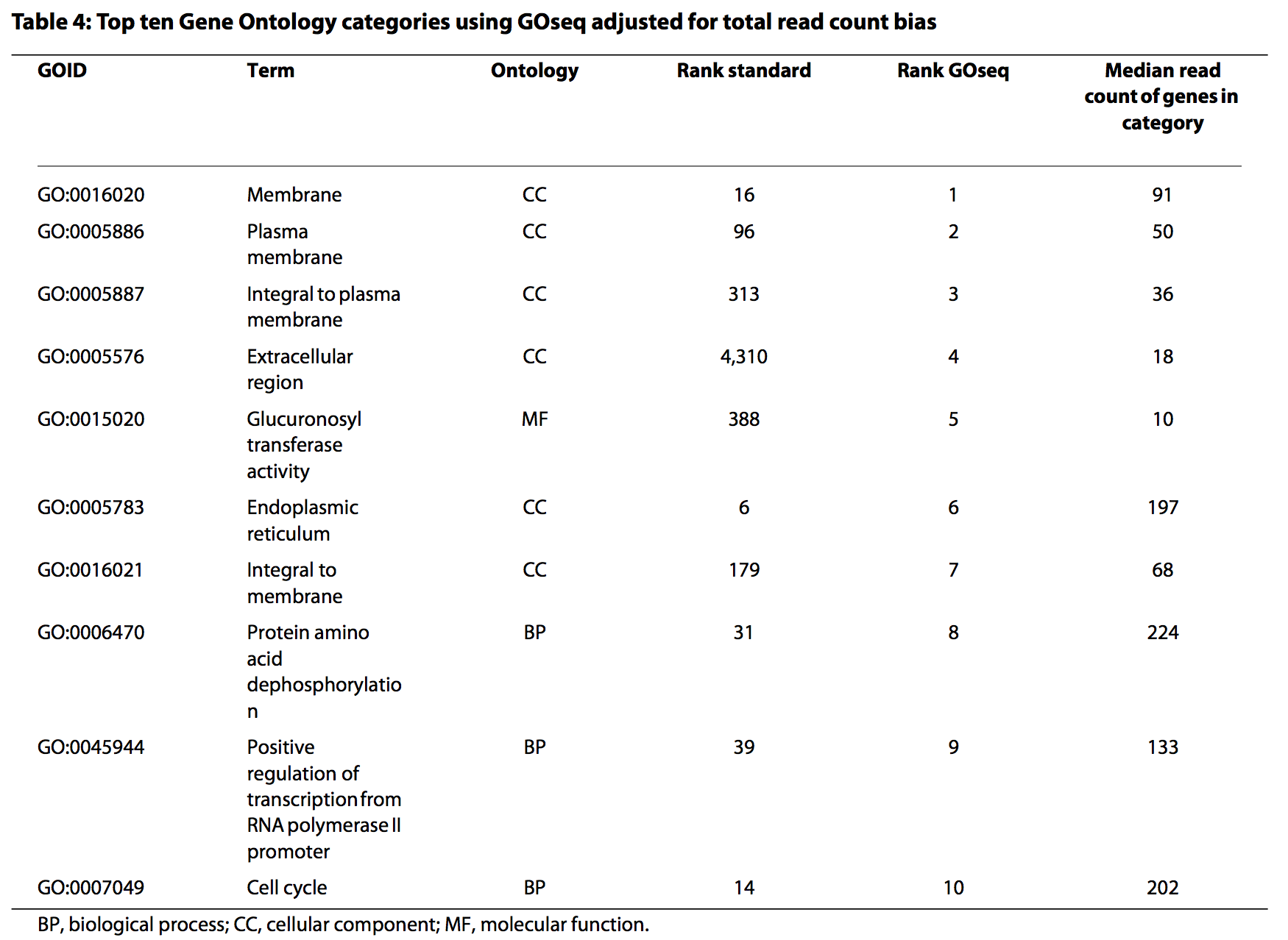
Results from the Young et al (2010) publication:
Proportion DE by gene length and reads
Gene set ranks by standard analysis
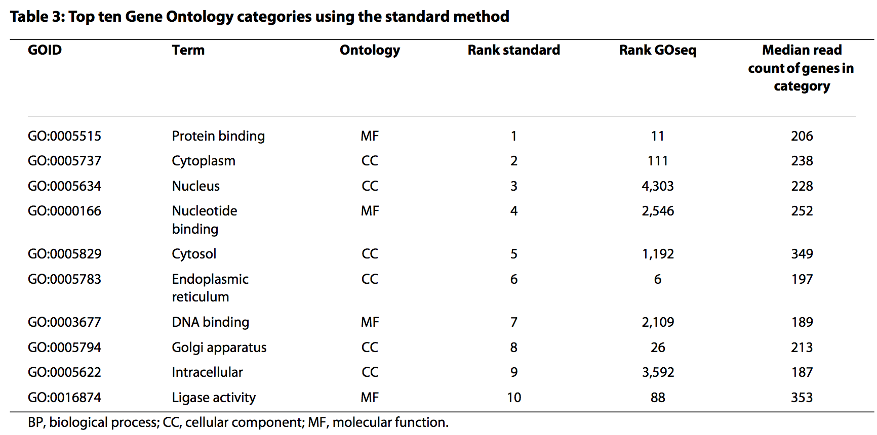
Gene set ranks by GOseq
GOseq analysis
Need to figure out if our organism is supported… (code is “sacCer”)
library(dplyr)
library(goseq)
supportedOrganisms() %>% head()
##          Genome         Id  Id Description Lengths in geneLeneDataBase
## 10      anoCar1    ensGene Ensembl gene ID                        TRUE
## 11      anoGam1    ensGene Ensembl gene ID                        TRUE
## 132     anoGam3                                                  FALSE
## 12      apiMel2    ensGene Ensembl gene ID                        TRUE
## 137 Arabidopsis                                                  FALSE
## 56      bosTau2 geneSymbol     Gene Symbol                        TRUE
##     GO Annotation Available
## 10                    FALSE
## 11                     TRUE
## 132                    TRUE
## 12                    FALSE
## 137                    TRUE
## 56                     TRUE
Easier to find if we use View() (NB - this only works in RStudio.
Can’t use in Jupyter on NeSI).
supportedOrganisms() %>% View()
Define differentially expressed genes
- Create a vector of 0’s and 1’s to denote whether or not genes are differentially expressed (limma analysis: topTable).
- Add gene names to the vector so that GOSeq knows which gene each data point relates to.
Load our topTable results from last session:
load('topTable.RData')
# Note: If you want to use tt from DESeq, replace $adj.P.Val with $padj below

genes <- ifelse(tt$adj.P.Val < 0.05, 1, 0)
names(genes) <- rownames(tt)
head(genes)
## YAL038W YOR161C YML128C YMR105C YHL021C YDR516C
##       1       1       1       1       1       1
table(genes)
## genes
##    0    1
## 1987 5140
Calculate gene weights
- Put genes into length-based “bins”, and plot length vs proportion differentially expressed
- Likely restricts to only those genes with GO annotation
pwf=nullp(genes, "sacCer1", "ensGene")

Inspect output
Report length (bias) and weight data per gene.
head(pwf)
    ##         DEgenes bias.data       pwf
    ## YAL038W       1      1504 0.8205505
    ## YOR161C       1      1621 0.8205505
    ## YML128C       1      1543 0.8205505
    ## YMR105C       1      1711 0.8205505
    ## YHL021C       1      1399 0.8205505
    ## YDR516C       1      1504 0.8205505
Gene lengths and weights
par(mfrow=c(1,2))
hist(pwf$bias.data,30)
hist(pwf$pwf,30)

Gene length vs average expression
Is there an association between gene length and expression level?
library(ggplot2)
data.frame(logGeneLength = log2(pwf$bias.data),
           avgExpr = tt$AveExpr) %>%
  ggplot(., aes(x=logGeneLength, y=avgExpr)) +
  geom_point(size=0.2) +
  geom_smooth(method='lm')

How about gene length and statistical evidence supporting differential expression?
(Kinda hard to see, but it is apparently there…)
data.frame(logGeneLength = log2(pwf$bias.data),
           negLogAdjP = -log10(tt$adj.P.Val)) %>%
  ggplot(., aes(x=logGeneLength, negLogAdjP)) +
  geom_point(size=0.2) +
  geom_smooth(method='lm')

Length correction in GOSeq
- Uses “Wallenius approximation” to perform correction.
- Essentially it is performing a weighted Fisher’s Exact Test, but each gene in the 2x2 data does not contribute equally to the per cell count - it instead contributes its weight (based on its length).
- This means that a gene set (e.g., GO term) containing lots of significant short genes will be considered more likely to be enriched that a gene set with a similar proportion of long genes that are differentially expressed.
Run GOSeq with gene length correction:
GO.wall=goseq(pwf, "sacCer1", "ensGene")
Output: Wallenius method
head(GO.wall)
    ##        category over_represented_pvalue under_represented_pvalue numDEInCat
    ## 1325 GO:0005622            1.817597e-17                        1       4298
    ## 7912 GO:0110165            8.200109e-12                        1       4456
    ## 5245 GO:0042254            9.441146e-12                        1        364
    ## 3817 GO:0022613            1.355385e-11                        1        439
    ## 5446 GO:0043226            2.516156e-11                        1       3826
    ## 5449 GO:0043229            4.433252e-11                        1       3817
    ##      numInCat                                 term ontology
    ## 1325     5179                        intracellular       CC
    ## 7912     5417           cellular anatomical entity       CC
    ## 5245      395                  ribosome biogenesis       BP
    ## 3817      482 ribonucleoprotein complex biogenesis       BP
    ## 5446     4609                            organelle       CC
    ## 5449     4599              intracellular organelle       CC
P-value adjustment
GO.wall.padj <- p.adjust(GO.wall$over_represented_pvalue, method="fdr")
sum(GO.wall.padj < 0.05)
## [1] 45
GO.wall.sig <- GO.wall$category[GO.wall.padj < 0.05]
length(GO.wall.sig)
## [1] 45
head(GO.wall.sig)
    ## [1] "GO:0005622" "GO:0110165" "GO:0042254" "GO:0022613" "GO:0043226"
    ## [6] "GO:0043229"
Filtering by gene set length
We are usually not interested in pathways or ontology terms that involve large numbers of genes (they are often rather broad terms or mechanisms), so we can exclude these from the results (here we only include significant GO terms that involve less than 500 genes):
GO.wall[GO.wall.padj < 0.05, ] %>% filter(numInCat < 500)
    ##      category over_represented_pvalue under_represented_pvalue numDEInCat
    ## 1  GO:0042254            9.441146e-12                1.0000000        364
    ## 2  GO:0022613            1.355385e-11                1.0000000        439
    ## 3  GO:0030684            3.348423e-08                1.0000000        163
    ## 4  GO:0016072            3.873737e-08                1.0000000        274
    ## 5  GO:0006364            4.532117e-08                1.0000000        259
    ## 6  GO:0034470            2.776978e-07                1.0000000        360
    ## 7  GO:0030490            9.891093e-07                0.9999998        111
    ## 8  GO:0030687            1.502461e-06                1.0000000         62
    ## 9  GO:0042274            2.616777e-06                0.9999993        134
    ## 10 GO:0005730            3.753501e-06                1.0000000        264
    ## 11 GO:0003735            3.799990e-06                1.0000000        194
    ## 12 GO:0022626            4.824970e-06                0.9999984        140
    ## 13 GO:0044391            6.732064e-06                1.0000000        202
    ## 14 GO:0000462            1.221128e-05                0.9999977         99
    ## 15 GO:0005840            1.780243e-05                0.9999942        221
    ## 16 GO:0002181            2.156069e-05                0.9999913        169
    ## 17 GO:0034660            7.782098e-05                0.9999571        409
    ## 18 GO:0042273            8.604282e-05                0.9999745        117
    ##    numInCat
    ## 1       395
    ## 2       482
    ## 3       171
    ## 4       299
    ## 5       282
    ## 6       401
    ## 7       116
    ## 8        62
    ## 9       143
    ## 10      292
    ## 11      221
    ## 12      156
    ## 13      231
    ## 14      104
    ## 15      254
    ## 16      191
    ## 17      467
    ## 18      126
    ##                                                                                        term
    ## 1                                                                       ribosome biogenesis
    ## 2                                                      ribonucleoprotein complex biogenesis
    ## 3                                                                               preribosome
    ## 4                                                                    rRNA metabolic process
    ## 5                                                                           rRNA processing
    ## 6                                                                          ncRNA processing
    ## 7                                                                    maturation of SSU-rRNA
    ## 8                                                      preribosome, large subunit precursor
    ## 9                                                        ribosomal small subunit biogenesis
    ## 10                                                                                nucleolus
    ## 11                                                       structural constituent of ribosome
    ## 12                                                                       cytosolic ribosome
    ## 13                                                                        ribosomal subunit
    ## 14 maturation of SSU-rRNA from tricistronic rRNA transcript (SSU-rRNA, 5.8S rRNA, LSU-rRNA)
    ## 15                                                                                 ribosome
    ## 16                                                                  cytoplasmic translation
    ## 17                                                                  ncRNA metabolic process
    ## 18                                                       ribosomal large subunit biogenesis
    ##    ontology
    ## 1        BP
    ## 2        BP
    ## 3        CC
    ## 4        BP
    ## 5        BP
    ## 6        BP
    ## 7        BP
    ## 8        CC
    ## 9        BP
    ## 10       CC
    ## 11       MF
    ## 12       CC
    ## 13       CC
    ## 14       BP
    ## 15       CC
    ## 16       BP
    ## 17       BP
    ## 18       BP
GO terms
- Can use the
GO.dbpackage to get more information about the significant gene sets.
library(GO.db)

GOTERM[[GO.wall.sig[1]]]
## GOID: GO:0005622
## Term: intracellular
## Ontology: CC
## Definition: The living contents of a cell; the matter contained within
##     (but not including) the plasma membrane, usually taken to exclude
##     large vacuoles and masses of secretory or ingested material. In
##     eukaryotes it includes the nucleus and cytoplasm.
## Synonym: internal to cell
## Synonym: protoplasm
## Synonym: nucleocytoplasm
## Synonym: protoplast
NB - the code below is demosntrating the difference between running with and without the gene length correction that GOseq implements. You wouldn’t usually work through this as part of a standard pathway analysis.
Run GOSeq without gene length correction
GO.nobias=goseq(pwf, "sacCer1", "ensGene", method="Hypergeometric")
Output: Hypergeomtric (Fisher) method
head(GO.nobias)
##        category over_represented_pvalue under_represented_pvalue numDEInCat
## 1325 GO:0005622            8.650971e-29                        1       4298
## 7912 GO:0110165            3.271100e-21                        1       4456
## 5446 GO:0043226            9.826546e-16                        1       3826
## 2650 GO:0009987            1.330459e-15                        1       4146
## 5449 GO:0043229            2.060920e-15                        1       3817
## 5245 GO:0042254            7.222008e-11                        1        364
##      numInCat                       term ontology
## 1325     5179              intracellular       CC
## 7912     5417 cellular anatomical entity       CC
## 5446     4609                  organelle       CC
## 2650     5023           cellular process       BP
## 5449     4599    intracellular organelle       CC
## 5245      395        ribosome biogenesis       BP
P-value adjustment
GO.nobias.padj <- p.adjust(GO.nobias$over_represented_pvalue, method="fdr")
sum(GO.nobias.padj < 0.05)
## [1] 44
GO.nobias.sig <- GO.nobias$category[GO.nobias.padj < 0.05]
length(GO.nobias.sig)
## [1] 44
head(GO.nobias.sig)
## [1] "GO:0005622" "GO:0110165" "GO:0043226" "GO:0009987" "GO:0043229"
## [6] "GO:0042254"
Compare with and without adjustment
library(gplots)
venn(list(GO.wall=GO.wall.sig, GO.nobias=GO.nobias.sig))

Extract out the different parts of the Venn diagram (yes, there are definitely better ways to do this).
## Only significant in Hypergeomtric analysis
onlySig.nobias <- setdiff(GO.nobias.sig, GO.wall.sig)

## Only significant in Wallenius analysis
onlySig.wall <- setdiff(GO.wall.sig, GO.nobias.sig)

## Significant in both
sig.wall.nobias <- intersect(GO.wall.sig, GO.nobias.sig)
Gene lengths and GO term membership
Can also extract gene length and GO membership information.
len=getlength(names(genes),"sacCer1","ensGene")

head(len)
## [1] 1504 1621 1543 1711 1399 1504
go = getgo(names(genes),"sacCer1","ensGene")

names(go) %>% head()
## [1] "YAL038W" "YOR161C" "YML128C" "YMR105C" "YHL021C" "YDR516C"
class(go)
## [1] "list"
head(go[[1]])
## [1] "GO:0006082" "GO:0008150" "GO:0008152" "GO:0009987" "GO:0019752"
## [6] "GO:0032787"
head(go[[2]])
## [1] "GO:0006810" "GO:0008150" "GO:0009987" "GO:0051179" "GO:0051234"
## [6] "GO:0055085"
Getting fancy…
Figure out which genes are in the significant GO groups, and then gets their lengths.
lengths.onlySig.nobias <- list()

for(i in 1:length(onlySig.nobias)){
  inGo <- lapply(go, function(x)  onlySig.nobias[i] %in% x) %>% unlist()
  lengths.onlySig.nobias[[i]] <- len[inGo]
}

lengths.onlySig.wall <- list()

for(i in 1:length(onlySig.wall)){
  inGo <- lapply(go, function(x)  onlySig.wall[i] %in% x) %>% unlist()
  lengths.onlySig.wall[[i]] <- len[inGo]
}
Significant: Hypergeometric vs Wallenius
- Only Hypergeometric (pink) vs only Wallenius (blue)
- Hypergeometric method is findings GO terms containing longer genes.
cols <- rep(c("lightpink", "lightblue"), c(10,7))
boxplot(c(lengths.onlySig.nobias, lengths.onlySig.wall), col=cols)

All significant GO terms
lengths.sig.wall.nobias <- list()

for(i in 1:length(sig.wall.nobias)){
  inGo <- lapply(go, function(x)  sig.wall.nobias[i] %in% x) %>% unlist()
  lengths.sig.wall.nobias[[i]] <- len[inGo]
}
cols <- rep(c("lightpink", grey(0.7), "lightblue"), c(10,37,7))

avgLength <- lapply(c(lengths.onlySig.nobias, lengths.sig.wall.nobias, lengths.onlySig.wall),
                    median) %>% unlist()

oo <- order(avgLength, decreasing=TRUE)
boxplot(c(lengths.onlySig.nobias, lengths.sig.wall.nobias, lengths.onlySig.wall)[oo],
        col=cols[oo], ylab="Gene Length", xlab = "GO term")

Gene length versus P-value
avgLength.wall <- lapply(c(lengths.onlySig.wall, lengths.sig.wall.nobias), median)

avgLength.nobias <- lapply(c(lengths.onlySig.nobias, lengths.sig.wall.nobias), median)

cols <- rep(c("blue", "lightblue", "red","lightpink"),
            c(length(lengths.onlySig.wall), length(lengths.sig.wall.nobias),
              length(lengths.onlySig.nobias), length(lengths.sig.wall.nobias)))

plot(c(avgLength.wall, avgLength.nobias),
     -log(c(GO.nobias.padj[GO.nobias.padj < 0.05], GO.wall.padj[GO.wall.padj < 0.05])),
     col=cols, pch=16, xlab="Median Gene Length", ylab ="-log(FDR adj-pval)")
legend('topright', c("Only sig in NoBias", "Sig in both (nobias adjp)",
                     "Sig in both (wal adjp)", "Only sig in Wall"),
       fill=c("red", "pink", "lightblue", "blue"))

Summary
- Once we’ve generated count data, there are a number of ways to perform a differential expression analysis.
- DESeq2 and edgeR model the count data, and assume a Negative Binomial distribution
- Limma transforms (and logs) the data and assumes normality
- Here we’ve seen that these three approches give quite similar results.
- For Gene Set analysis, gene length needs to be accounted for, since
longer transcripts are more likely to be found to be differentially
expressed.
- GOSeq adjusts for transcript length to take this into account.
- It is also possible to use GOSeq with other types of annotation (e.g., Reactome or KEGG pathways).
Key Points
Coordinated changes in groups of functionally related genes can tell us about the underlying biological mechanisms that changing between exprimental conditions.
The characteristics of RNA-seq experiments mean that gene-length correction is required, to avoid standard approaches to over-representation analysis givign erroneous results.