Map and count reads
Overview
Teaching: 45 min
Exercises: 0 minQuestions
How do we turn fastq data into read counts?
Objectives
Align reads to reference genome.
Assess read mapping for each sample.
Generate per-sample count data for each genomic feature (e.g., genes, exons etc) that you are interested in.
Alignment to a reference genome
RNA-seq generate gene expression information by quantifying the number of transcripts (per gene) in a sample. This is acompished by counting the number of transcripts that have been sequenced - the more active a gene is, the more transcripts will be in a sample, and the more reads will be generated from that transcript.
For RNA-seq, we need to align or map each read back to the genome, to see which gene produced it.
- Highly expressed genes will generate lots of transcripts, so there will be lots of reads that map back to the position of that transcript in the genome.
- The per-gene data we work with in an RNA-seq experiment are counts: the number of reads from each sample that originated from that gene.
Preparation of the genome
To be able to map (align) sequencing reads on the genome, the genome needs to be indexed first. In this workshop we will use HISAT2. Note for speed reason, the reads will be aligned on the chr5 of the mouse genome.
$ cd /home/[Your_Username]/obss_2021/RNA_seq/Genome

#to list what is in your directory:
$ ls /home/[Your_Username]/obss_2021/RNA_seq/Genome
Saccharomyces_cerevisiae.R64-1-1.99.gtf Saccharomyces_cerevisiae.R64-1-1.dna.toplevel.fa
$ module load HISAT2/2.2.0-gimkl-2020a

# index file:
$ hisat2-build -p 4 -f Saccharomyces_cerevisiae.R64-1-1.dna.toplevel.fa Saccharomyces_cerevisiae.R64-1-1.dna.toplevel

#list what is in the directory:
$ ls /home/[Your_Username]/obss_2021/RNA_seq/Genome
Saccharomyces_cerevisiae.R64-1-1.99.gtf              Saccharomyces_cerevisiae.R64-1-1.dna.toplevel.4.ht2  Saccharomyces_cerevisiae.R64-1-1.dna.toplevel.8.ht2
Saccharomyces_cerevisiae.R64-1-1.dna.toplevel.1.ht2  Saccharomyces_cerevisiae.R64-1-1.dna.toplevel.5.ht2  Saccharomyces_cerevisiae.R64-1-1.dna.toplevel.fa
Saccharomyces_cerevisiae.R64-1-1.dna.toplevel.2.ht2  Saccharomyces_cerevisiae.R64-1-1.dna.toplevel.6.ht2
Saccharomyces_cerevisiae.R64-1-1.dna.toplevel.3.ht2  Saccharomyces_cerevisiae.R64-1-1.dna.toplevel.7.ht2
Option info:
- -p number of threads
- -f fasta file
How many files were created during the indexing process?
Alignment on the genome
Now that the genome is prepared. Sequencing reads can be aligned.
Information required:
- Where the sequence information is stored (e.g. fastq files …) ?
- What kind of sequencing: Single End or Paired end ?
- Where are stored the indexes and the genome?
-
Where will the mapping files be stored?
- Now, lets move one folder up (into the RNA_seq folder):
$ cd ..

$ ls
Genome QC Raw Trimmed
Let’s map one of our sample to the genome
$ hisat2 -x Genome/Saccharomyces_cerevisiae.R64-1-1.dna.toplevel -U Raw/SRR014335-chr1.fastq -S SRR014335.sam
125090 reads; of these:
  125090 (100.00%) were unpaired; of these:
    20537 (16.42%) aligned 0 times
    85066 (68.00%) aligned exactly 1 time
    19487 (15.58%) aligned >1 times
83.58% overall alignment rate
Now we need to align all the rest of the samples.
$ pwd
/home/[Your_Username]/obss_2021/RNA_seq/
$ mkdir Mapping

$ ls
Genome Mapping QC Raw SRR014335.sam Trimmed
let’s use a for loop to process our samples:
$ cd Trimmed

$ ls
SRR014335-chr1.fastq SRR014336-chr1.fastq SRR014337-chr1.fastq SRR014339-chr1.fastq SRR014340-chr1.fastq SRR014341-chr1.fastq
$ for filename in *.trimmed.fastq
> do
> base=$(basename ${filename} .trimmed.fastq)
> hisat2 -p 4 -x ../Genome/Saccharomyces_cerevisiae.R64-1-1.dna.toplevel -U $filename -S ../Mapping/${base}.sam --summary-file ../Mapping/${base}_summary.txt
> done
Now we can explore our SAM files.
$ cd ../Mapping

$ ls
SRR014335-chr1.sam          SRR014336-chr1_summary.txt  SRR014339-chr1.sam          SRR014340-chr1_summary.txt
SRR014335-chr1_summary.txt  SRR014337-chr1.sam          SRR014339-chr1_summary.txt  SRR014341-chr1.sam
SRR014336-chr1.sam          SRR014337-chr1_summary.txt  SRR014340-chr1.sam          SRR014341-chr1_summary.txt
Converting SAM files to BAM files
The SAM file, is a tab-delimited text file that contains information for each individual read and its alignment to the genome. While we do not have time to go into detail about the features of the SAM format, the paper by Heng Li et al. provides a lot more detail on the specification.
The compressed binary version of SAM is called a BAM file. We use this version to reduce size and to allow for indexing, which enables efficient random access of the data contained within the file.
A quick look into the sam file
$ less SRR014335-chr1.sam
The file begins with a header, which is optional. The header is used to describe the source of data, reference sequence, method of alignment, etc., this will change depending on the aligner being used. Following the header is the alignment section. Each line that follows corresponds to alignment information for a single read. Each alignment line has 11 mandatory fields for essential mapping information and a variable number of other fields for aligner specific information. An example entry from a SAM file is displayed below with the different fields highlighted.
We will convert the SAM file to BAM format using the samtools program with the view command and tell this command that the input is in SAM format (-S) and to output BAM format (-b):
$ module load SAMtools/1.10-GCC-9.2.0

$ for filename in *.sam
> do
> base=$(basename ${filename} .sam)
> samtools view -S -b ${filename} -o ${base}.bam
> done

$ ls
SRR014335-chr1.bam  SRR014336-chr1.bam  SRR014337-chr1.bam  SRR014339-chr1.bam  SRR014340-chr1.bam  SRR014341-chr1.bam
SRR014335-chr1.sam  SRR014336-chr1.sam  SRR014337-chr1.sam  SRR014339-chr1.sam  SRR014340-chr1.sam  SRR014341-chr1.sam
Sorting BAM files
Next we sort the BAM file using the sort command from samtools. -o tells the command where to write the output.
$ for filename in *.bam
> do
> base=$(basename ${filename} .bam)
> samtools sort -o ${base}_sorted.bam ${filename}
> done
SAM/BAM files can be sorted in multiple ways, e.g. by location of alignment on the chromosome, by read name, etc. It is important to be aware that different alignment tools will output differently sorted SAM/BAM, and different downstream tools require differently sorted alignment files as input.
You can use samtools to learn more about the bam file as well.
Some stats on your mapping:
$ samtools flagstat SRR014335-chr1_sorted.bam
156984 + 0 in total (QC-passed reads + QC-failed reads)
31894 + 0 secondary
0 + 0 supplementary
0 + 0 duplicates
136447 + 0 mapped (86.92% : N/A)
0 + 0 paired in sequencing
0 + 0 read1
0 + 0 read2
0 + 0 properly paired (N/A : N/A)
0 + 0 with itself and mate mapped
0 + 0 singletons (N/A : N/A)
0 + 0 with mate mapped to a different chr
0 + 0 with mate mapped to a different chr (mapQ>=5)
MultiQC: HISAT2 output
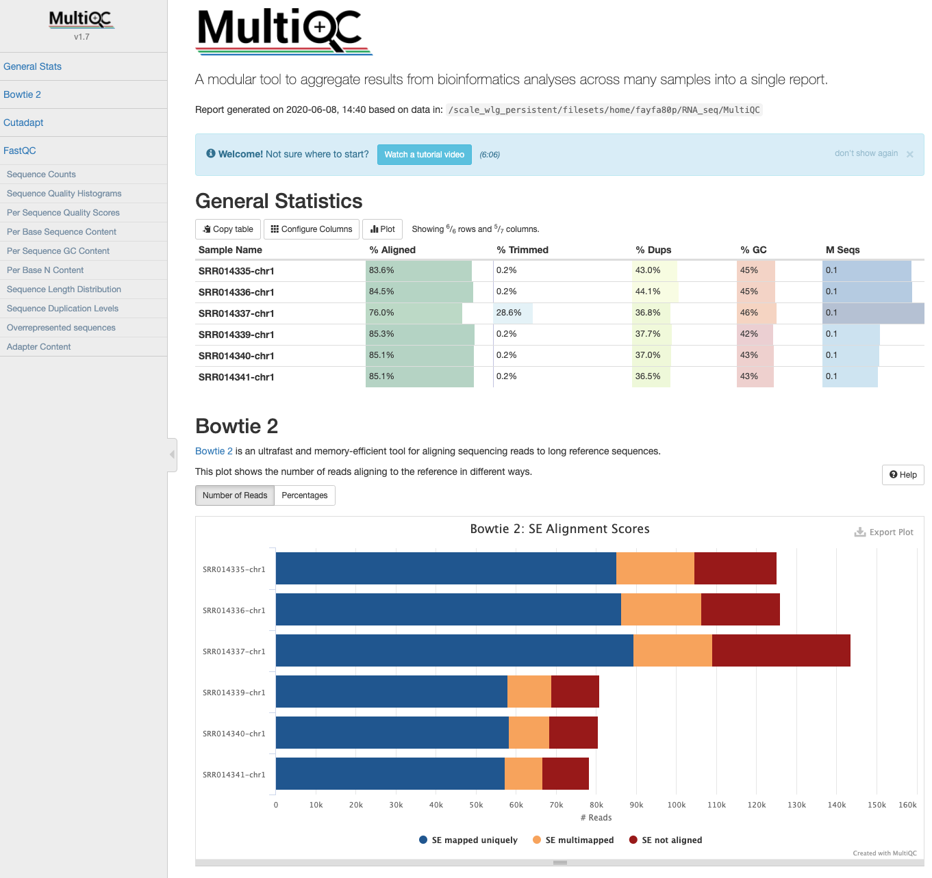
- The HISAT2 output data can also be incorporated into the MultiQC report the next time it is run.
 $ cd ~/obss_2021/RNA_seq/MultiQC

 $ cp ../Mapping/*summary* ./

 $ multiqc .

Please note: running HISAT2 with either option --summary-file or older versions (< v2.1.0) gives log output identical to Bowtie2. These logs are indistinguishable and summary statistics will appear in MultiQC reports labelled as Bowtie2.
Read Summarization
Sequencing reads often need to be assigned to genomic features of interest after they are mapped to the reference genome. This process is often called read summarization or read quantification. Read summarization is required by a number of downstream analyses such as gene expression analysis and histone modification analysis. The output of read summarization is a count table, in which the number of reads assigned to each feature in each library is recorded.
Counting
- We need to do some counting!
- Want to generate count data for each gene (actually each exon) - how many reads mapped to each exon in the genome, from each of our samples?
- Once we have that information, we can start thinking about how to determine which genes were differentially expressed in our study.
Subread and FeatureCounts
- The featureCounts tool from the Subread package can be used to count how many reads aligned to each genome feature (exon).
- Need to specify the annotation informatyion (.gtf file) You can process all the samples at once:
$ module load Subread

$ pwd
/home/[Your_Username]/obss_2021/RNA_seq

$ mkdir Counts

$ cd Counts

$ featureCounts -a ../Genome/Saccharomyces_cerevisiae.R64-1-1.99.gtf -o ./yeast_counts.txt -T 2 -t exon -g gene_id ../Mapping/*sorted.bam
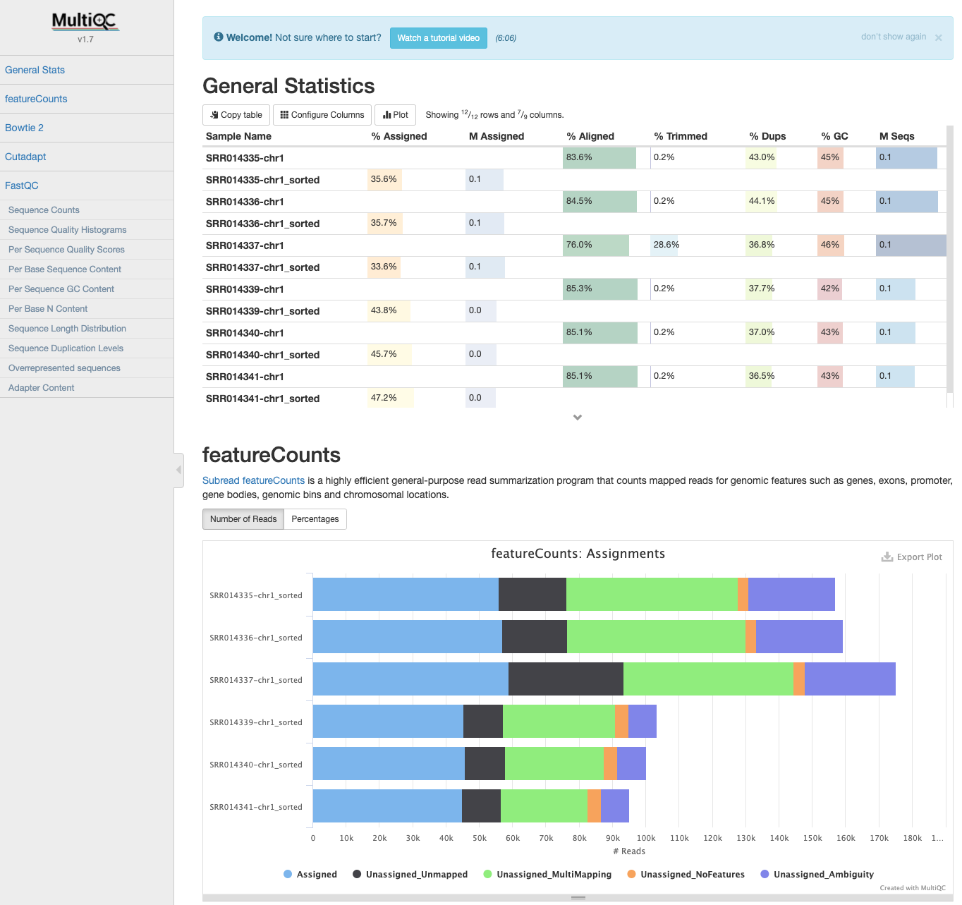
MultiQC: featureCounts output
- If the samples are processed individually, the output data can be incorporated into the MultiQC report the next time it is run.
$ cd ../MultiQC

$ cp ../Counts/* .

$ multiqc .

Since we now have all the count data in one file, we need to transfer it to our local computers so we could start working on RStudio to get differentially expressed genes.
- And the code to do it is below, however for this workshop, we are going to use a different file (yeast_counts_all_chr.txt) that you can download from section 4. Differential_Expression. This file has all the data for all the chromosomes.
#In a new terminal that you can access you computer files, cd to the directory you want to save the counts file.

$ scp fayfa80p@login.mahuika.nesi.org.nz:/home/fayfa80p/RNA_seq/Counts/yeast_counts_all_chr.txt ./
Download with Jupyter
An alternative is to navigate to the directory
~/obss_2021/RNA_seq/Counts/in the navigation panel of Jupyter then right-click onyeast_counts_all_chr.txtand select “Download”
Key Points
Alignment and feature counting are used to generate read counts for each genomic feature (e.g., genes) of interest, per sample.
The count data can then be used for stataistical analysis (e.g., to identify differentially expressed genes).