Metabarcoding Basics
Overview
Teaching: 15 min
Exercises: 0 minQuestions
What are the main components of metabarcoding pipelines?
Objectives
Review typical metabarcoding workflows
eDNA Workshop
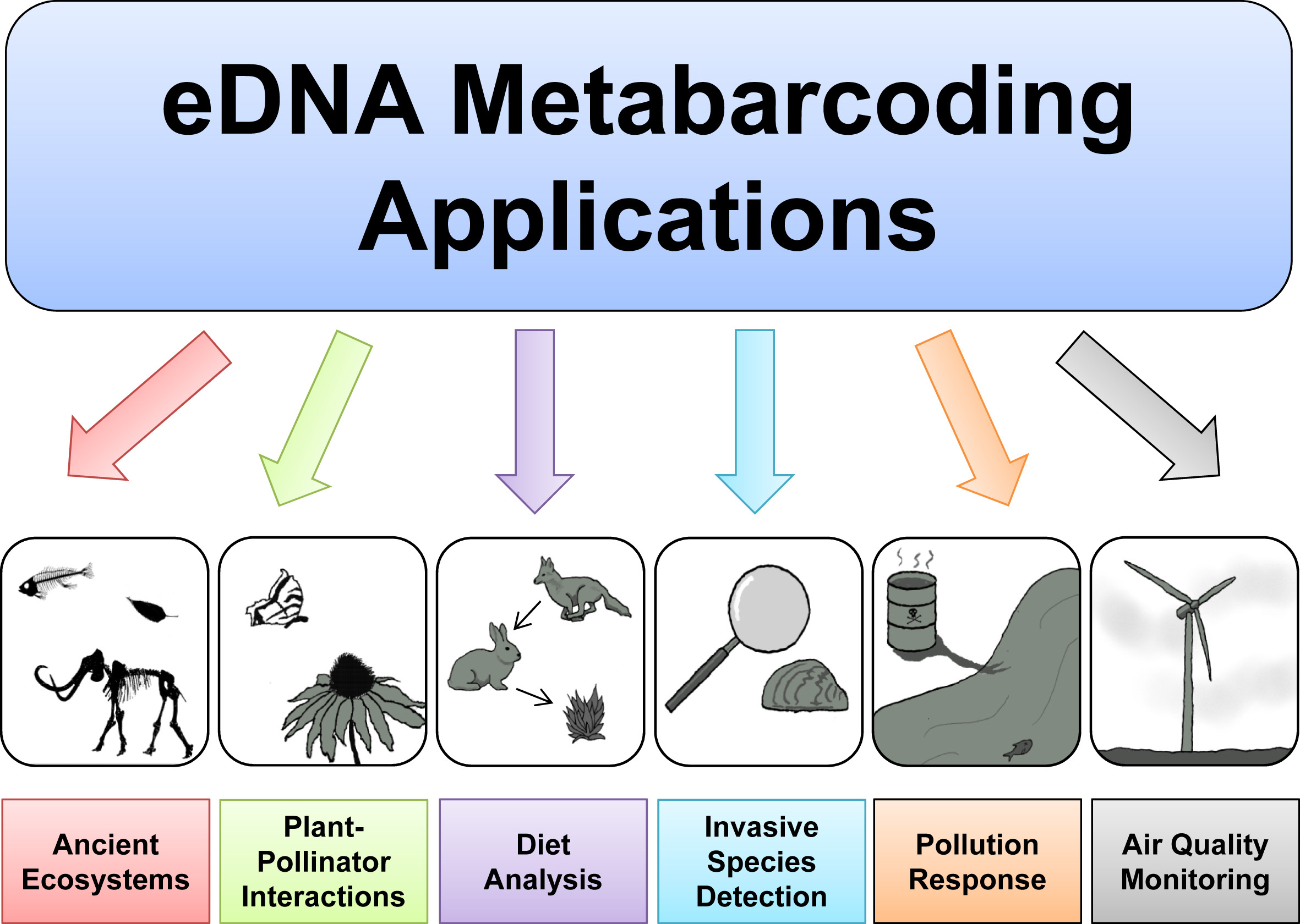
The primary goal of this course is to introduce students to the analysis of environmental DNA data. The set of methods that broadly has to do with the analysis of nucleic material from the environment is called Metagenomics. Usually this refers to shotgun metagenomics, which utilises shotgun next-generation sequencing (NGS). However, there are several techniques used nowadays for analysing eDNA, including bait capture, qPCR, and metatranscriptomics (eRNA). This course will cover eDNA metabarcoding , which involves using PCR amplification of one or a few genes on DNA extracted from environmental samples.
Major software programs used for eDNA metabarcoding
There are a number of software packages and pipelines that are available for eDNA metabarcoding (hereafter referred to as just metabarcoding). We will go over several of these programs in the course of this workshop. It would be inpractical to cover all of them, but one of the objectives of this course is to show the student how to interact with multiple programs without getting too bogged down. We feel it is important to keep a flexible approach so that the student ultimately has more tools at their disposal. We will only cover a handful of programs here, but hopefully you will leave the course having learned how to learn a new program. You will see all the steps from raw data to publication-quality graphs.
Some of the major programs for metabarcoding (those marked with a ‘*’ will be covered in this workshop):
-
Qiime2* is actually a collection of different programs and packages, all compiled into a single ecosystem so that all things can be worked together. On the Qiime2 webpage there is a wide range of tutorials and help. We will use this program to do the taxonomy analyses, but we will also show you how to easily import and export from this format so you can combine with other programs.
-
Dada2 is a good program, run in the R language. There is good documentation and tutorials for this on its webpage. You can actually run Dada2 within Qiime, but there are a few more options when running it alone in R.
-
USEARCH (webpage), and the open-source version (which we will use) (VSEARCH*), has many utilities for running metabarcoding analyses. Many of the most common pipelines use at least some of the tools from these packages.
-
Mothur has long been a mainstay of metabarcoding analyses, and is worth a look
-
Another major program for metabarcoding is OBITools, which was one of the first to specialise in non-bacterial metabarcoding datasets. The newer version, updated for Python 3, is currently in Beta. Check the main webpage to keep track of its development.
Additionally, there are several good R packages that we will use to analyse and graph our results. Chief among these are Phyloseq* and DECIPHER*.
Metabarcoding Basics
Most metabarcoding pipelines and software use similar tools and methodological approaches, and there are a common set of file types. The methods and the underlying concepts will be presented as we go through the example sets, but to start off, here we introduce a basic tool kit for metabarcoding (aside from the specific software packages themselves), and review the basic file types and formats that will be used for this course, and for most metabarcoding. If you have a firm grasp of these files, then it will be easier to transform your data so it can be used with almost any metabarcoding software package.
Basic tool kit
-
The terminal, aka Command Line Interface (CLI).
-
A text editor. Two of the best that can work on any platform are Sublime Text and Visual Studio Code. For Macs, BBEdit is a popular choice. And for Windows, Notepad++ is tried and true. Atom is a good open source option.
-
RStudio, an all-in-one package for R.
Building blocks of metabarcoding
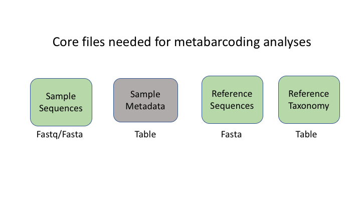
There are six basic kinds of information that are common to all metabarcoding analyses. In some programs, the information may be combined into fewer files. In other programs, such as Qiime2, the files are largely separate. For the purposes of clarity, we will present these as separate files.
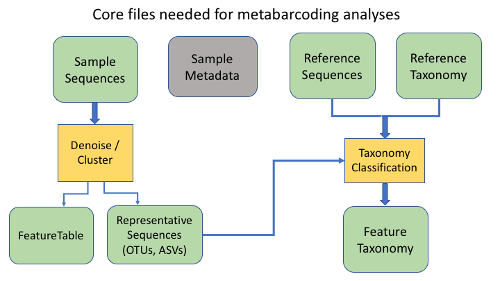
The first two data types have to do with your sample data: your sequence data, and the metadata holding information about each sample. The next two are for the taxonomic references that are used to determine the species composition of the samples.
Sequence files: fastq and fasta
The first files are fastq and fasta files. You have seen many examples of this file type already this week.
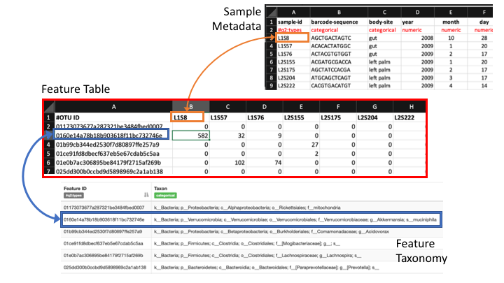
Sample Metadata
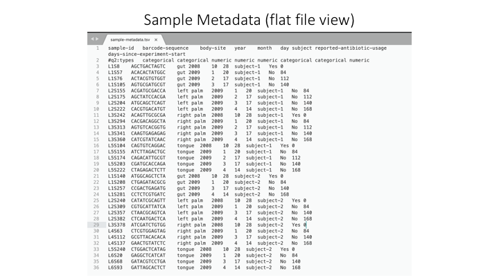
The sample metadata will have different formats, depending on the programs used, but usually is a simple tab-delimited file with information for each sample:
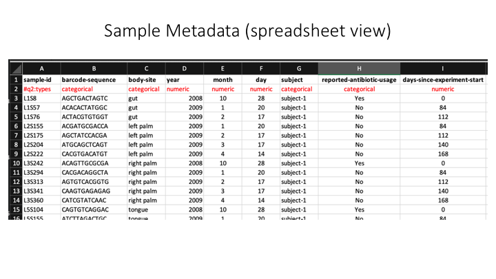
Here is a spreadsheet view, so the different categories are clearer:
Now we will open the sample metadata file that we will use in this course. In JupyterHub, navigate to the docs folder. You will see a file called sample_metadata.tsv. Double-click on this file and it will open in a new tab on Jupyter. You will see that Jupyter recognises this file as a table, because of the .tsv suffix.
Taxonomy files
The format of taxonomy files varies depending on the program you are running. Most programs combine this information into a fasta file with the lineage information on the sequence id line. For example, in Sintax (run with VSEARCH), the program we will be using, the format looks like this:
>MW856870;tax=k:Eukaryota,p:Chordata,c:Actinopteri,o:Perciformes,f:Percidae,g:Percina,s:Percina_roanoka
ACAAGACAGATCACGTTAAACCCTCCCTGACAAGGGATTAAACCAAATGAAACCTGTCCTAATGTCTTTGGTTGGGGCGACCGCGGGGAAACAAAAAACCCCCACGTGGA...
In Qiime, there are two files: one is a fasta file with the reference sequences.
>MW856870
ACAAGACAGATCACGTTAAACCCTCCCTGACAAGGGATTAAACCAAATGAAACCTGTCCTAATGTCTTTGGTTGGGGCGACCGCGGGGAAACAAAAAACCCCCACGTGGA...
This is accompanied by a taxonomy table that shows the taxonomic lineage for each sequence ID:
MW856870 d__Eukaryota;p__Chordata;c__Actinopteri;o__Perciformes;f__Percidae;g__Percina;s__Percina_roanoka
OTU files
The next two information types come after clustering the sample sequences. The clustered sequences are also known as Operational Taxonomic Units (OTUs), Amplicon Sequence Variants (ASVs), Exact Sequence Variants (ESVs), or zero radius OTUs (zOTUs), depending on how they are produced (e.g. clustering or denoising). The last type is a frequency table that specifies how many sequences of each OTU are found in each sample. (The general Qiime2 terminology for these are the representative sequences and the feature table.)
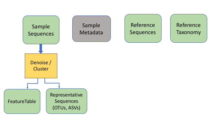
To keep things simple, we will refer to all of these types as OTUs, as that is the oldest and most widely recognised term.
An additional important data type is the product of taxonomy classification of the representative sequences, here called the feature taxonomy
Frequency tables are key to metabarcoding analyses
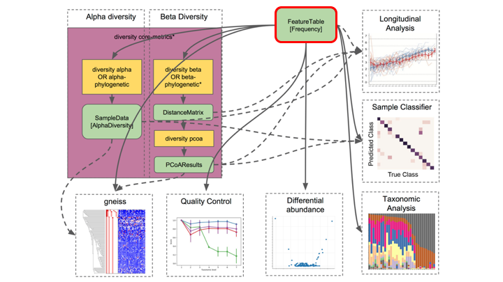
The frequency table (or feature table) ties together many sources of information in your analysis. It combines the per sample frequencies of each OTU, and to its taxonomic assignment, and these in turn can be linked to the sample metadata.
Frequency Tables are the centre of multiple downstream analyses
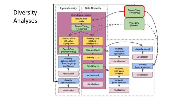
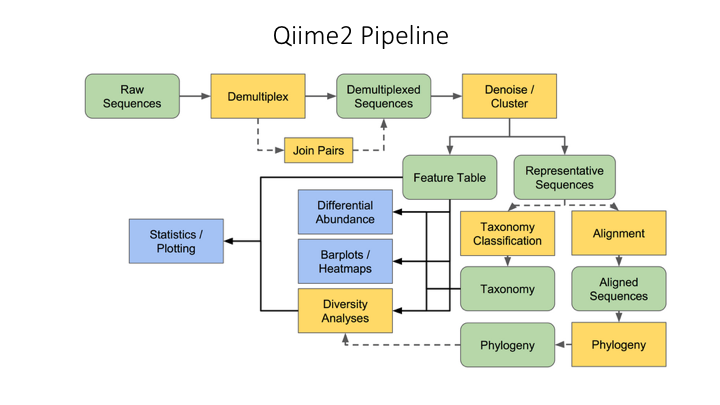
Typical metabarcoding pipelines
Most metabarcoding workflows have mostly the same steps. The Qiime webpage has a good illustration of their pipeline:
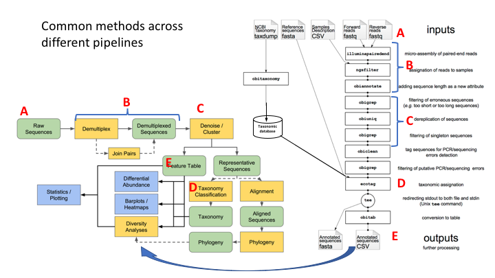
Here are the OBITools and Qiime pipelines side-by-side. Though the steps are named somewhat differently, the methods employed are very similar.
Tour of project subfolders
For any project, it is important to organise your various files into subfolders. Through the course you will be navigating between folders to run your analyses. It may seem confusing or tedious, especially as there are only a few files. Remember that for many projects you can easily generate hundreds of files, so it is best to start with good practices from the beginning.
Your edna folder is located in ~/obss_2021/. It has the following subfolders:
- docs/
- data/
- otus/
- taxonomy/
- scripts/
- plots/
- notebooks/
- references/
Most of these are empty, but by the end of the course they will be full of the results of your analysis.
Before we begin, you need to copy a file to your scripts folder:
cp /nesi/project/nesi02659/obss_2021/resources/day4/eDNA.sh ~/obss_2021/edna/scripts
This file contains instructions to load all the paths and modules you will need for the rest of the day. You will see how it works in the next lesson.
Key Points
Most metabarcoding pipelines include the same basic components
Frequency tables are key to metabarcoding analyses
Demultiplexing and Trimming
Overview
Teaching: 20 min
Exercises: 10 minQuestions
What are the different primer design methods for metabarcoding?
How do we demultiplex and quality control metabarcoding data?
Objectives
Learn the different methods for QC of metabarcoding data
Initial processing of raw sequence data
We will start where almost any data analysis begins (after creating metadata files of course), processing our raw data file.
Amplicon primer design
There are many ways to design metabarcoding primers to amplify your region of your interest from environmental samples. We will not cover too much experimental design in this course, but the way the experiment was set up will always influence how you approach the analysis.
Here are two common methods.
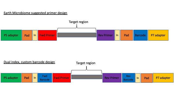
The first design above comes from the Earth Microbiome project (EMP). In this method, the sequencing center will usually do the demultiplexing for you, because the barcode is in a region recognised by Illumina standard protocols. We will not cover this, but in these cases, you will get back a folder of multiple fastq sequence files, one for each sample (barcode).
In the second case above, there are two barcodes, one on the forward primer (P5 adapter side) and one on the reverse (P7 adapter side). The advantage of this method, called dual index, is that it allows you to use the two barcodes in combination so you have fewer overall barcode-primers to order. However, you will need to demultiplex these sequences yourself. The example dataset uses this method.
The next consideration is whether the sequencing method was paired end or single end. For paired end sequencing libraries, in the case of the EMP method, for each sample you will have one file for the forward sequence and one for the reverse; for the dual index strategy, you will have two files total, that will have to be demultiplexed in tandem. Usually in metabarcoding, after demultiplexing and filtering, the two pairs are merged together (and any that cannot be merged are not used). This is different from other types of NGS sequencing, like genome assembly or RNAseq, where the pairs are kept separate.
The example dataset for today was created with single end sequencing, so there is just a single file.
In order to use our data, we will have to clean it up by removing the primers and any sequence upstream or downstream of the primers, then filtering out any sequences that are too short or of low average quality. If the data has not been split into separate files for each sample, then we will need to also demultiplex the raw data file.
To get started, navigate to the data/ subfolder within the ~/obss_2021/edna/ directory.
$ cd ~/obss_2021/edna
$ pwd
/home/username/obss_2021/edna
Assuming you are in the main directory:
$ cd data
and then use the ls command to see the contents of the subfolder
$ ls -lh
-rwxrwx---+ 1 hugh.cross nesi02659 119M Nov 20 04:25 FTP103_S1_L001_R1_001.fastq.gz
The h option in the ls command stands for human readable. This option will show the size of large files as MB (megabytes) or GB (gigabytes), instead of a long string of numbers representing the number of bytes.
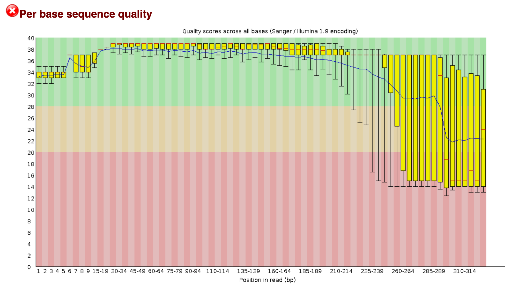
You remember on Day 2 we went over FastQC. On the course page there is an image from a FastQC sequence quality data run on this file. You will see that the file still has a lot of poor quality sequence that have to be removed.
Demultiplexing, trimming, and quality filtering
For the single-end, dual-indexed sequences that we are using today, we will need to demultiplex the raw fastq file. We also need to trim the primers and filter out low-quality reads. Fortunately, to avoid confusion we have written a short program that will do these steps for us. This program is freely available on the GitHub page. As well, on the workshop website, there are example commands for each of the steps.
The program, cutadaptQC, will read the primer and barcode sequences from the sample metadata file, and use these to create a new sequence file for each sample, which we can use for downstream analyses. It will also create a fasta file (without the quality information) for each final, filtered fastq file. Finally, the program will run FastQC on each final fastq file and then a program called MultiQC which combines all the separate FastQC files into one webpage.
As with other programs you have seen, this program has options that you view with the -h argument. Before we can view the help documentation, we will need to navigate to the scripts folder and source the eDNA.sh file. This will load the module in our environment.
cd ../scripts/
source eDNA.sh
cutadaptQC -h
usage: cutadaptQC [-h] [-m METADATAFILE] [-r FASTQ] [-f DATAFOLDER] [-l MIN_LENGTH] [-x MAX_LENGTH] [-a MAXN]
                  [-e ERROR] [-n PROJECTNAME] [-t THREADS]

Run cutadapt to demultiplex and quality control raw sequence data

optional arguments:
  -h, --help            show this help message and exit

arguments:
  -m METADATAFILE, --metadata_file METADATAFILE
                        sample metadata file
  -r FASTQ, --raw_fastq FASTQ
                        Raw data file to be processed
  -f DATAFOLDER, --data_folder DATAFOLDER
                        Folder to process sequence data
  -l MIN_LENGTH, --min_length MIN_LENGTH
                        [OPTIONAL] minimum length for reads (default:150)
  -x MAX_LENGTH, --max_length MAX_LENGTH
                        [OPTIONAL] maximum length for reads (default:300)
  -a MAXN, --max_n MAXN
                        [OPTIONAL] maximum number of Ns in sequence (default:0)
  -e ERROR, --error ERROR
                        [OPTIONAL] maximum expected error value (default:1.0)
  -n PROJECTNAME, --name PROJECTNAME
                        [OPTIONAL] Name of project (default:"fish")
  -t THREADS, --threads THREADS
                        [OPTIONAL] number of CPUs to use (default:1)
Because there are a few options to add here, we will be running this program using a bash script, As we have done on Day 2 and 3 of this workshop.
Build a script to run the program cutadaptQC
To start, we will navigate to the scripts folder if you are not there already. Then, we will open a new file by using the
nanotext editor that is incorporated into the terminal. When we run this command, it will open a new file wherein we can write our code.nano trim_qc.shHints: First, you need to tell the script what modules to load so all software can be accessed. All of the modules that need to load are incorporated into the
eDNA.shfile.source eDNA.shNow, we can add the actual command to the script. When we ran the help command for this program, it gave us the options we need to input along with the name of the program. There are several parameters we are required to fill in and others (with a default option) are only needed if the default values do not suit your specific requirements. I recommend following the options in the help documentation, to make sure that you do not forget to enter one of the parameters.
-m: the program needs the metadata file to know which barcode and primer sequences to use for each sample. This file can be find in thedocs/folder, so we need to remember to add the (relative) path.
-r: indicates the raw sequencing file (FTP103_S1_L001_R1_001.fastq.gz), which is located in thedata/folder.
-f: indicates the folder where all the processed files will be stored. Today, we will use thedata/folder.
-n: for the project name, we will usefish_project, given the sequencing data represents the fish diversity observed at Otago Harbour.
-t: we can set the number of threads to 4.We can leave the default values for all other options, as the
minimumandmaximumlength are within our amplicon range, Illumina sequencing data should not haveNbasecalls, and theerror rateof 1.0 is a standard approach in processing metabarcoding data.We can exit out of
nanoby pressingctr+x, followed byyandenterto save the file.Solution
Your script should look like this:
source eDNA.sh

cd ~/obss_2021/edna

cutadaptQC \
 -m ./docs/sample_metadata.tsv \
 -r ./data/FTP103_S1_L001_R1_001.fastq.gz \
 -f ./data \
 -n fish_project \
 -t 4 \
Now, to run this script, in the terminal run it like this:
$ bash trim_qc.sh
If it works, then you should see the outputs begin to be generated. This will take a a minute or two to run. While this is running, in the Folder tab, you can navigate over to the data folder, where you should see new subfolders with the trimmed fastq and fasta files.
Once the script has finished, you should have five new subfolders in your data/ folder:
- trimmed
- fastq
- fasta
- fastq_qc
- {Project Name}_multiqc_report_data
The trimmed/ subfolder has the fastq sequence files from which primers and barcode sequences have been removed. There is now one for each sample. The fastq/ folder has the fastq sequence files files, in which each file has taken the corresponding trimmed file and run a quality filter and removed any sequences below the minimum length. The fasta files in the fasta/ are from the fastq files, from which any quality information has been removed. The fastq_qc folder contains all the FastQC output, and the {Project Name}_multiqc_report_data folder (substitute your project name for {Project Name}).
In addition to these folders, you also have a web file that is the multiQC report: {Project Name}_multiqc_report.html. Go ahead and double click on this file to open it. Once opened, you will see what looks like a FastQC file, but one that has the combined results for all the files. In the upper part of the file, there is text that says Trust HTML. Click on this to see all the figures in the graph (This is a security precaution for Jupyter).
In the terminal, we can have a peek at some of the other files:
$ cd ../data/fastq

$ head -n 12 AM1_filt.fastq
@AM1.1
GAAAGGTAGACCCAACTACAAAGGTCCCCCAATAAGAGGACAAACCAGAGGGACTACTACCCCCATGTCTTTGGTTGGGGCGACCGCGGGGGAAGAAGTAACCCCCACGTGGAACGGGAGTACAACTCCTTGAACTCAGGGCCACAGCTCTAAGAAACAAAATTTTTGACCTTAAGATCCGGCAATGCCGATCAACGGACCG
+
2E2AEHHFHFGGEGGEHFGHGHGCFFEGGEFDGHHEFFEFGGGFFFE1CGGGGFGCGHGHHGGECHFHFHHHGGHHGGGGFCGCCGFCCGGGGGGHHG0CGHHHDCFFCGEGBFFGDFD?DBBFFBFFFFFFFFFFFFFE?DDDEFFFFFFFFFFFFFFFFFFFFFFAEFFFFFFFFFFFFFF;BFFFFFFFFDBFDADCFF
@AM1.2
ACAAGGCAGCCCCACGTTAAAAAACCTAAATAAAGGCCTAAACTTACAAGCCCCTGCCCTTATGTCTTCGGTTGGGGCGACCGCGGGGTAAAAAATAACCCCCACGTGGAATGGGGGCATAAACACCCCCCCAAGTCAAGAGTTACATCTCCAGGCAGCAGAATTTCTGACCATAAGATCCGGCAGCGCCGATCAGCGAACCA
+
HH4FHHGGGGFGDEEEHHFEFFFGGGHHFHHEFHHEFGHHHFGHHHHGFHGFHGHEEHHHHHHHHFHHFEEGGGGGGGCGCG/B?CFGFGHHHHGHHHHHHGGGGGGAADFG0B?DGGGGGFGGGFDFGFFFFF.BBFFFFFFFFFFFFFFFFFEEEDFF.BFFFFFFFEFFFFFFFFFFFFFFCFFFFFFFFFDFFFFFFFF
@AM1.3
ACAAGGCAGCCCCACGTTAAAAAACCTAAATAAAGGCCTAAACTTACAAGCCCCTGCCCTTATGTCTTCGGTTGGGGCGACCGCGGGGTAAAAAATAACCCCCACGTGGAATGGGGGCATAAACACCCCCCCAAGTCAAGAGTTACATCTCCAGGCAGCAGAATTTCTGACCATAAGATCCGGCAGCGCCGATCAGCGAACCA
+
HH4AGHHGGDGEEGA?GHFGFHGFGFHGHHHFHHGGGFHGFGHHHFHHFFHFGGHEGFGFHHHGHFFHFGGGGGGGGGGGGG?@/CFGGGHHHHGHHHHHHGGGFGCCEDGG0FEFGGGGFBFGGFDDGCFAFF?FFFFFEFBBFFEFFFFFFFFFEFFF;BBFFFFFF/FFFFFFFFFFFFFFAFFFFFFFFFFFFFFFFFF
Key Points
First key point. Brief Answer to questions. (FIXME)
Denoising or clustering the sequences
Overview
Teaching: 15 min
Exercises: 30 minQuestions
Is it better to denoise or cluster sequence data?
Objectives
Learn to cluster sequences into OTUs with the VSEARCH pipeline
Introduction
Now that our sequences have been trimmed and filtered, we can proceed to the next step, which will create a set of representative sequences. We do this by clustering all the sequences to look for biologically meaningful sequences, those that are thought to represent actual taxa, while trying to avoid differences caused by sequence or PCR errors, and remove any chimeric sequences.
Scientists are currently debating on what the best approach is to obtain biologically meaningful or biologically correct sequences. There are numerous papers published on this topic. Unfortunately, this is something that is outside the scope of this workshop to go into at depth. But here is the basic information…
There are basically two trains of thought, clustering the dataset or denoising the dataset. With clustering the dataset, an OTU (Operational Taxonomic Unit) sequence should be at least a given percentage different from all other OTUs and should be the most abundant sequence compared to similar sequences. People traditionally chose to cluster at 97%, which means that the variation between sequences should be at least 3%. The concept of OTU clustering was introduced in the 1960s and has been debated ever since. With denoising the dataset, on the other hand, the algorithm attempts to identify all correct biological sequences in the dataset, which is visualized in the figure below. This schematic shows a clustering threshold at 100% and trying to identify errors based on abundance differences. The retained sequences are called ZOTU or Zero-radius Operational Taxonomic Unit. In other software programs they might also be called ASVs.
For purposes of clarity, we will call all these representative sequences OTUs, as that is the most common and oldest term for this type.
This difference in approach may seem small but has a very big impact on your final dataset!
When you denoise the dataset, it is expected that one species may have more than one ZOTU, while if you cluster the dataset, it is expected that an OTU may have more than one species assigned to it. This means that you may lose some correct biological sequences that are present in your data when you cluster the dataset, because they will be clustered together. In other words, you will miss out on differentiating closely related species and intraspecific variation. For denoising, on the other hand, it means that when the reference database is incomplete, or you plan to work with ZOTUs instead of taxonomic assignments, your diversity estimates will be highly inflated.
For this workshop, we will follow the clustering pathway, since most people are working on vertebrate datasets with good reference databases and are interested in taxonomic assignments.
Prior to clustering or denoising, we need to dereplicate our data into unique sequences. Since metabarcoding data is based on an amplification method, the same starting DNA molecule can be sequenced multiple times. In order to reduce file size and computational time, it is convenient to combine these duplicated sequences as one and retain information on how many were combined. Additionally, we will remove sequences that only occur once in our data and attribute them to sequence and PCR error. Lastly, we will sort the sequences based on abundance.
Before we do all of this, we need to combine all of the fasta files into a single file. In the terminal, navigate to the data/fasta/ folder:
$ cd ~/obss_2021/edna/data/fasta
Now we will just concatenate all the fasta files into one using the cat command:
$ cat *.fasta > combined.fasta
For the actual dereplication, size sorting, and clustering, we will be running these commands using bash scripts. Therefore, we need to navigate back to the scripts/ folder and create a new script.
$ cd ../../scripts
Build a script to dereplicate the data and sort sequences based on abundance
Similarly to the previous script, we will use the
nanotext editor to generate the.shfilenano dereplicate_seqs.shFor this and the next scripts, we will use the program VSEARCH (https://github.com/torognes/vsearch). To load this module, we can source the
eDNA.shfile, as you did in the previous script.source eDNA.shRemember that the bash script is being executed from the
scriptsfolder. Since we want to save our OTUs in theotusfolder, we will need to indicate this in the script.In this bash script, we will run two commands: one to
dereplicatethe sequences and another tosortthe sequences by abundance. Below, you can find the two commands for this. Please note that in a bash script we can run commands sequentially by putting them one after another. Also note how the second command uses an input file that was generated as an output file in the first command.vsearch --derep_fulllength "INPUT_FILENAME_1" --minuniquesize 2 --sizeout --output "OUTPUT_FILENAME_1" --relabel Uniq. vsearch --sortbysize "OUTPUT_FILENAME_1" --output "OUTPUT_FILENAME_2"Similarly to what we did during the first bash script, we can exit out of
nanoby pressingctr+x, followed byyandenterto save the file.Remember that to run the script, we use
bash, followed by the filename.bash dereplicate_seqs.shSolution
Your script should look like this:
source eDNA.sh

cd ../otus/

vsearch --derep_fulllength ../data/fasta/combined.fasta \
--minuniquesize 2 \
--sizeout \
--output derep_combined.fasta \
--relabel Uniq.

vsearch --sortbysize derep_combined.fasta \
--output sorted_combined.fasta
To check if everything executed properly, we can list the files that are in the otus folder and check if both output files have been generated (derep_combined.fasta and sorted_combined.fasta).
$ ls -ltr ../otus/
-rw-rw----+ 1 hugh.cross nesi02659 545795 Nov 24 03:52 derep_combined.fasta
-rw-rw----+ 1 hugh.cross nesi02659 545795 Nov 24 03:52 sorted_combined.fasta
We can also check how these commands have altered our files. Let’s have a look at the sorted_combined.fasta file, by using the head command.
$ head ../otus/sorted_combined.fasta
>Uniq.1;size=19583
TTTAGAACAGACCATGTCAGCTACCCCCTTAAACAAGTAGTAATTATTGAACCCCTGTTCCCCTGTCTTTGGTTGGGGCG
ACCACGGGGAAGAAAAAAACCCCCACGTGGACTGGGAGCACCTTACTCCTACAACTACGAGCCACAGCTCTAATGCGCAG
AATTTCTGACCATAAGATCCGGCAAAGCCGATCAACGGACCG
>Uniq.2;size=14343
ACTAAGGCATATTGTGTCAAATAACCCTAAAACAAAGGACTGAACTGAACAAACCATGCCCCTCTGTCTTAGGTTGGGGC
GACCCCGAGGAAACAAAAAACCCACGAGTGGAATGGGAGCACTGACCTCCTACAACCAAGAGCTGCAGCTCTAACTAATA
GAATTTCTAACCAATAATGATCCGGCAAAGCCGATTAACGAACCA
>Uniq.3;size=8755
ACCAAAACAGCTCCCGTTAAAAAGGCCTAGATAAAGACCTATAACTTTCAATTCCCCTGTTTCAATGTCTTTGGTTGGGG
Study Questions
What do you think the following parameters are doing?
--sizeout--minuniquesize 2--relabel Uniq.Solution
--sizeout: this will print the number of times a sequence has occurred in the header information. You can use theheadcommand on the sorted file to check how many times the most abundant sequence was encountered in our sequencing data.
--minuniquesize 2: only keeps the dereplicated sequences if they occur twice or more. To check if this actually happened, you can use thetailcommand on the sorted file to see if there are any dereplicates sequences with--sizeout 1.
--relabel Uniq.: this parameter will relabel the header information toUniq.followed by an ascending number, depending on how many different sequences have been encountered.
Now that we have dereplicated and sorted our sequences, we can cluster our data, remove chimeric sequences, and generate a frequency table. We will do this by generating our third script
Build a script to generate a frequency table
Again, we will use the
nanotext editor to generate the.shfilenano cluster.shWe will be using VSEARCH again for all three commands, so we will need to source the
eDNA.shfile in our script.source eDNA.shRemember that the bash script is being executed from the
scriptsfolder. For all three commands, we will output the generated files in theotusfolder. Therefore, we will need to indicate this in the bash script.In this bash script, we will run three commands: one to
clusterthe sequences using a user-specified similarity threshold, one to removechimericsequences, and one to generate afrequencytable. Below, you can find all three commands that we will use.vsearch --cluster_size "OUTPUT_FILENAME_2" --centroids "OUTPUT_FILENAME_3" --sizein --id 0.97 --sizeout vsearch --uchime3_denovo "OUTPUT_FILENAME_3" --sizein --fasta_width 0 --nonchimeras "OUTPUT_FILENAME_4" --relabel OTU. vsearch --usearch_global "INPUT_FILENAME_1" --db "OUTPUT_FILENAME_4" --id 0.97 --otutabout "OUTPUT_FILENAME_5"Similarly to what we did during the first bash script, we can exit out of
nanoby pressingctr+x, followed byyandenterto save the file.Remember that to run the script, we use
bash, followed by the filename.bash cluster.shSolution
Your script should look like this:
source eDNA.sh

cd ../otus/

vsearch --cluster_size sorted_combined.fasta \
--centroids centroids.fasta \
--sizein \
--id 0.97 \
--sizeout

vsearch --uchime3_denovo centroids.fasta \
--sizein \
--fasta_width 0 \
--nonchimeras otus.fasta \
--relabel OTU.

vsearch --usearch_global ../data/fasta/combined.fasta \
--db otus.fasta \
--id 0.97 \
--otutabout otu_frequency_table.tsv
Tip
Check the example commands above, do you need to change any paths?
Study Questions
The results of the last script creates three files:
centroids.fasta,otus.fasta, andotu_frequency_table.tsv. Let’s have a look at these files to see what the output looks like. From looking at the output, can you guess what some of these VSEARCH parameters are doing?
--sizein--sizeout--centroids--relabelHow about
--fasta_width 0? Try rerunning the script without this command to see if you can tell what this option is doing.Hint: you can always check the help documentation of the module by loading the module
source eDNA.shand calling the help documentationvsearch -hor by looking at the manual of the software, which can usually be found on the website.
Optional extra 1
We discussed the difference between denoising and clustering. You can change the last script to have VSEARCH do clustering instead of denoising. Make a new script to run clustering. It is similar to
cluster.sh, except you do not use thevsearch --cluster_unoisecommand. Instead you will use:vsearch --cluster_unoise sorted_combined.fasta --sizein --sizeout --fasta_width 0 --centroids centroids_unoise.fastaYou will still need the commands to remove chimeras and create a frequency table. Make sure to change the names of the files so that you are making a new frequency table and OTU fasta file (maybe call it
asvs.fasta). If you leave the old name in, it will be overwritten when you run this script.Give it a try and compare the number of OTUs between clustering and denoising outputs.
Optional extra 2
The
--idargument is critical for clustering. What happens if you raise or lower this number? Try rerunning the script to see how it changes the results. Note: make sure to rename the output each time or you will not be able to compare to previous runs.
Key Points
Clustering sequences into OTUs can miss closely related species
Denoising sequences can create overestimate diversity when reference databases are incomplete
Taxonomy Assignment
Overview
Teaching: 15 min
Exercises: 30 minQuestions
What are the main strategies for assigning taxonomy to OTUs?
What is the difference between Sintax and Naive Bayes?
Objectives
Assign taxonomy using Sintax
Use
lessto explore a long help outputWrite a script to assign taxonomy
Taxonomy Assignment: Different Approaches
There are four basic strategies to taxonomy classification (and endless variations of each of these): sequence similarity (SS), sequence composition (SC), phylogenetic (Ph), and probabilistic (Pr) (Hleap et al., 2021).
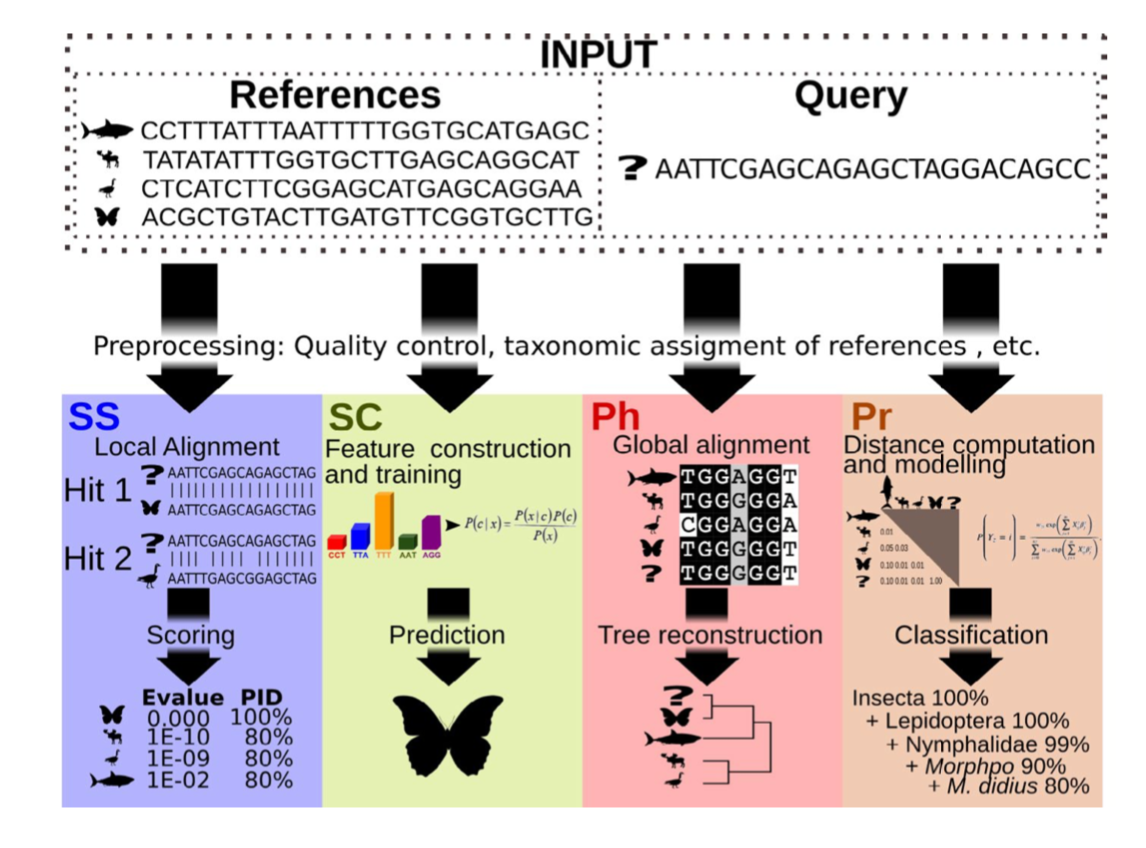
Of the four, the first two are those most often used for taxonomy assignment. For further comparison of these refer to this paper.
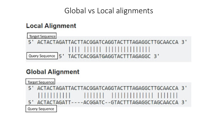
Aligment-Based Methods (SS)
All sequence similarity methods use global or local alignments to directly search a reference database for partial or complete matches to query sequences. BLAST is one of the most common methods of searching DNA sequences. BLAST is an acronym for Basic Local Alignment Search Tool. It is called this because it looks for any short, matching sequence, or local alignments, with the reference. This is contrasted with a global alignment, which tries to find the best match across the entirety of the sequence.
Using Machine Learning to Assign Taxonomy
Sequence composition methods utilise machine learning algorithms to extract compositional features (e.g., nucleotide frequency patterns) before building a model that links these profiles to specific taxonomic groups.

Use the program Sintax to classify our OTUs
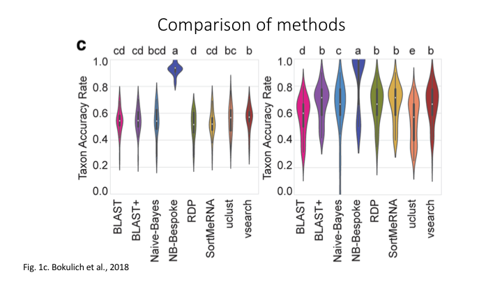
The program Sintax is similar to the Naive Bayes classifier used in Qiime and other programs, in that small 8 bp kmers are used to detect patterns in the reference database, but instead of frequency patterns, k-mer similarity is used to identify the top taxonomy, so there is no need for training (Here is a description of the Sintax algorithm). Because of this, it is simplified and can run much faster. Nevertheless, we have found it as accurate as Naive Bayes for the fish dataset we are using in this workshop.
As with the previous steps, we will be using a bash script to run the classification. As before, we will use VSEARCH to run Sintax.
Go to the scripts folder and create a file called classify_sintax.sh, using either Nano (nano classify_sintax.sh) or from the Launcher in Jupyter.
To access any program needed for this workshop, first source the eDNA.sh file
source eDNA.sh
The VSEARCH command has many functions and many options. In the command line, you can list these more easily using less:
vsearch -h | less
Looking at a long help command this way allows you to scroll up and down the help options. For the sintax script, you will need to fill in these parameters:
--sintax--db--sintax_cutoff--tabbedout
Write a script to run sintax through VSEARCH
Hints:
Start to fill in the neccessary components. We will go through each of the arguments.
When you start searching with
less, you can quit anytime by just enteringq.You can also search for a specific part of the help output by entering a forward slash (
/), followed by the term you are looking forYou can go to top of the search by entering
gg, and to the bottom by enteringG.Try to figure out which parameter you need to fill in for each of these options.
To get you started, the
--sintaxargument has to go right aftervsearch, and its parameter is the name of the OTU file you created in the last lessonSolution
source ~/obss_2021/edna/scripts/eDNA.sh

cd ~/obss_2021/edna/taxonomy/

vsearch --sintax \
 ../otus/otus.fasta \
 --db ../references/aramoana_ref_db.fasta \
 --sintax_cutoff 0.8 \
 --tabbedout sintax_raw_taxonomy.tsv
After the first line, we just put the name of the OTU file from the clustering lesson, remember the path is needed to point the program to where the file is
On the next line, after the
--db, put the path../references/and the reference file.The next line is for the confidence cut off. If the estimated confidence of a taxonomic assignment falls below this number, the assignment will not be recorded. » The default for this is 0.6, but we will use a higher cutoff of
0.8for the--sintax_cutoffargument.The final line is to name the output file. You can use any name, but it is better to include some information such as the name of the OTUs and program used » (sintax), in case want to compare the results with other runs. Also include the suffix
.tsv, which will tell Jupyter that it is a table file.
Now you are done. Save and close the file. Then run it on the command line.
bash classify_sintax.sh
Have a look at the output file. Find the file in the taxonomy folder and double click to open it in Jupyter. You will see it is divided into two main parts. The first includes the name of each rank (e.g. p:Chordata to indicate the phylum Chordata), followed by the confidence for the assignment at that rank in parentheses. The second section, which follows the +, has only the name of each rank and includes only those ranks whose confidence is above the --sintax_cutoff parameter used.
Study Questions
Name an OTU that would have better resolution if the cutoff were set to default
Name an OTU that would have worse resolution if the cutoff were set higher
Visualisation in Qiime
In Qiime, all the visuals are run as interactive web apps–they need to run on a web browser. In this course we will focus on creating graphs and plots using R. However, we have provided some links to visuals for the OTUs and taxonomy for this data set, in order to show how some of the visuals work.
For all these plots, they need to be opened on a webpage called Qiime2View. Click on the following link to open it in a new tab:
To see a table of the taxonomy assignment of each OTU, paste the following link into the Qiime2View webpage (do not click on it).
https://otagoedna.github.io/2019_11_28_edna_course/example_viz/fish_NB_taxonomy_VIZ.qzv
Then go to the Qiime2View website, click on ‘file from the web’, and paste the link in the box that opens up.
The next plot is a barplot graph of the taxonomy. A barplot graph is a good way to compare the taxonomic profile among samples.
Paste the following link into the Qiime2View page:
https://otagoedna.github.io/2019_11_28_edna_course/example_viz/fish_NB_taxonomy_barplot.qzv
We are also including a table of the OTU sequences.
https://otagoedna.github.io/2019_11_28_edna_course/example_viz/zotus_tabulation.qzv
This visual shows the sequence for each OTU. You can run a BLAST search on each OTU by clicking on the sequence. However, the search can take a while, depending on how busy the NCBI server is.
Converting the output file
While the sintax output file is very informative, we will convert it to a simpler format that will make it easier to import into other downstream applications. Fortunately, the eDNA module has a script that will convert the file into several other formats. At the terminal prompt, go to the taxonomy folder and enter the script name and the help argument
convert_tax2table.py -h
You will see the options:
usage: convert_tax2table.py [-h] [-i INPUT] [-o OUTPUT] [-f FORMAT]

Convert taxonomy output to tabular format

optional arguments:
  -h, --help            show this help message and exit

arguments:
  -i INPUT, --input_file INPUT
                        Input taxonomy file to convert
  -o OUTPUT, --output_table OUTPUT
                        Name of output table
  -f FORMAT, --format FORMAT
                        Format of input file, options: "sintax","idtaxa","qiime"; default=sintax
This program will run very fast, so you can run it on the command line. Check the output. You should see a new table with each taxonomic rank in its own column. (Hint: if you name the output file with .tsv at the end, then it will open in Jupyter as a table.)
cd ../taxonomy

convert_tax2table.py -i sintax_raw_taxonomy.tsv -o sintax_taxonomy.tsv
Extra exercise: use IDTaxa for taxonomy assignment
There are many methods available for taxonomy assignment. Another popular option is IDTaxa. IDTaxa is a variant of the RDP machine learning approach, discussed above.
Write a bash script to run this program.
Guide:
- IDTaxa requires the reference data to be trained. We have made a pre-trained classifier available for you in the
/referencessubfolder.- IDTaxa is a R package from the Bioconductor library, so you will need to load the Bioconductor R bundle, which will also load R:
module load R-bundle-Bioconductor/3.13-gimkl-2020a-R-4.1.0- To run this on the command line, there is an R script in the
/scriptssubfolder that will run IDTaxa, and then convert the output to a table:run_IDTaxa.R- To run a R script from the command line or a bash script, you need to use the command
RScript --vanilla, followed by the name of the script.- For this R script, the arguments come after the script and have to be entered in this order:
Rscript --vanilla run_IDTaxa.R <IDTaxa_classifier> <otu_fasta> <output_file>Solution
Your script should contain these lines (assuming you are running it from the scripts folder)
module purge
module load R-bundle-Bioconductor/3.13-gimkl-2020a-R-4.1.0

Rscript --vanilla \
  run_IDTaxa.R \
  ../references/fish_lrRNA_idtaxa_classifier.rds \
  ../otus/otus.fasta \
  ../taxonomy/idtaxa_taxonomy.tsv
Note that you do not have to split this across separate lines with a
\, but it helps to read the code.
Key Points
The main taxonomy assignment strategies are global alignments, local alignments, and machine learning approaches
The main difference is that Naive Bayes requires the reference data to be trained, whereas Sintax looks for only kmer-based matches
Creating A Reference Database
Overview
Teaching: 15 min
Exercises: 30 minQuestions
What reference databases are available for metabarcoding
How do I make a custom database?
Objectives
First learning objective. (FIXME)
Reference databases
As we have previously discussed, eDNA metabarcoding is the process whereby we amplify a specific gene region of the taxonomic group of interest from an environmental sample. Once the DNA is amplified, we sequence it and up till now, we have been filtering the data based on quality and assigned sequences to samples. The next step in the bioinformatic process will be to assign a taxonomy to each of the sequences, so that we can determine what species are detected through our eDNA analysis.
There are multiple ways to assign taxonomy to a sequence. While this workshop won’t go into too much detail about the different taxonomy assignment methods, any method used will require a reference database.
Several reference databases are available online. The most notable ones being NCBI, EMBL, BOLD, SILVA, and RDP. However, recent research has indicated a need to use custom curated reference databases to increase the accuracy of taxonomy assignment. While certain reference databases are available (RDP: 16S microbial; MIDORI: COI eukaryotes; etc.), this necessary data source is missing in most instances.
Hugh and I, therefore, developed a python software program that can generate custom curated reference databases for you, called CRABS: Creating Reference databases for Amplicon-Based Sequencing. While we will be using it here in the workshop, it is unfortunately not yet publicly available, since we are currently writing up the manuscript. However, we hope that we can release the program by the end of this year. We hope this software program will provide you with the necessary tools to help you generate a custom reference database for your specific study!
CRABS - a new program to build custom reference databases
The CRABS workflow consists of seven parts, including:
- (i) downloading and importing data from online repositories into CRABS;
- (ii) retrieving amplicon regions through in silico PCR analysis;
- (iii) retrieving amplicons with missing primer-binding regions through pairwise global alignments using results from in silico PCR analysis as seed sequences;
- (iv) generating the taxonomic lineage for sequences;
- (v) curating the database via multiple filtering parameters;
- (vi) post-processing functions and visualizations to provide a summary overview of the final reference database; and
- (vii) saving the database in various formats covering most format requirements of taxonomic assignment tools.
Today, we will build a custom curated reference database of fish sequences from the 16S gene region. Once we’ve completed this reference database, you could try building your own shark reference database from the 16S gene region or try the taxonomy assignment of your OTUs with this newly generated reference database to see how it performs.
Before we get started, we will quickly go over the help information of the program. As before, we will first have to source the eDNA.sh script to load the program.
source eDNA.sh
crabs_v1.0.1 -h
usage: crabs_v1.0.1 [-h] {db_download,db_import,db_merge,insilico_pcr,pga,assign_tax,dereplicate,seq_cleanup,geo_cleanup,visualization,tax_format} ...

creating a curated reference database

positional arguments:
  {db_download,db_import,db_merge,insilico_pcr,pga,assign_tax,dereplicate,seq_cleanup,geo_cleanup,visualization,tax_format}

optional arguments:
  -h, --help            show this help message and exit
As you can see, the help documentation shows you how to use the program, plus displays all the 11 functions that are currently available within CRABS. If you would want to display the help documentation of a function, we can type the following command:
crabs_v1.0.1 db_download -h
usage: crabs_v1.0.1 db_download [-h] -s SOURCE [-db DATABASE] [-q QUERY] [-o OUTPUT] [-k ORIG] [-e EMAIL] [-b BATCHSIZE]

downloading sequence data from online databases

optional arguments:
  -h, --help            show this help message and exit
  -s SOURCE, --source SOURCE
                        specify online database used to download sequences. Currently supported options are: (1) ncbi, (2) embl, (3) mitofish, (4) bold, (5)
                        taxonomy
  -db DATABASE, --database DATABASE
                        specific database used to download sequences. Example NCBI: nucleotide. Example EMBL: mam*. Example BOLD: Actinopterygii
  -q QUERY, --query QUERY
                        NCBI query search to limit portion of database to be downloaded. Example: "16S[All Fields] AND ("1"[SLEN] : "50000"[SLEN])"
  -o OUTPUT, --output OUTPUT
                        output file name
  -k ORIG, --keep_original ORIG
                        keep original downloaded file, default = "no"
  -e EMAIL, --email EMAIL
                        email address to connect to NCBI servers
  -b BATCHSIZE, --batchsize BATCHSIZE
                        number of sequences downloaded from NCBI per iteration. Default = 5000
Step 1: download sequencing data from online repositories
During this workshop, you will not have to run this command, since the file has been provided to you!
When we look at the help documentation of the
db_downloadfunction, we can see that CRABS let’s us download sequencing data from 4 repositories using the--sourceparameter, including:
- NCBI
- BOLD
- EMBL
- MitoFish
Today, we will be downloading 16S fish sequences from NCBI. According to the help documentation, we will need to fill out multiple parameters.
--source: online repository to download sequencing data from.
--database: sequencing database of NCBI to download sequences from.
--query: NCBI query search that encompasses the data you would like to download. This query is based on thesearch detailsbox on the NCBI website (https://www.ncbi.nlm.nih.gov/nuccore). Let’s have a look at this now!
--output: output filename.
The code to download the 16S sequences of sharks would look for example like this:
crabs_v1.0.1 db_download \
--source ncbi \
--database nucleotide \
--query '16S[All Fields] AND ("Chondrichthyes"[Organism] OR Chondrichthyes[All Fields]) AND ("1"[SLEN] : "50000"[SLEN])' \
--output 16S_chondrichthyes_ncbi.fasta \
--email johndoe@gmail.com
Rather than everyone downloading sequencing data off NCBI at the same time, we will copy a sequencing file from the resources/day folder in our references folder. This file named ncbi_16S.fasta is the file generated by the db_download function and contains all 16S sequences on NCBI that are assigned to Animalia.
cp /nesi/project/nesi02659/obss_2021/resources/day4/ncbi_16S.fasta ~/obss_2021/edna/references
Let’s look at the top 10 lines of the sequencing file to determine the format.
head -10 ../references/ncbi_16S.fasta
>EF646645
ATTTAGCTAGTAACAGCAAGCAAAACGCAATTTTAGTTTGCACCCCCGAAACTAAGTGAGCTACTTTAAAACAGCCATATGGGCCAACTCGTCTCTGTTGCAAAAGAGTGAGAAGATTTTTAAGTAGAAGTGACAAGCCTATCGAACTTAGAGATAGCTGGTTATTTGGGAAAAGAATATTAGTTCTGCCTTAAGCTTTTATTAACACCCTTCAAAGCAACTTAAGAGTTATTCAAATAAGGTACAGCCTATTTGATACAGGAAACAACCTAAAACATAGGGTAACGCTACCTACAATTTTTATAATTAAGTTGGCCTAAAAGCAGCCATCTTTTAAAAAGCGTCAAAGCTTAATTATTTAATAACAACAATCACAACAAAAATGCCAAACCCACCACTACTACCAAATAACTTTATATAATTATAAAAGATATTATGCTAAAACTAGTAATAAGAAAATGACTTTCTCCTAAATATAAGTGTAATGCAGAATAAACAAATCACTGCTAATTATTGTTTTTGATTAAATAGTAGCAACCTCTCTAGAAAACCCTACTATAAATAACATTAACCTAACACAAGAATATTACAGGAAAAATTAAAAG
>EF646644
ATTTAGCTAGTCAAAACAAGCAAAGCGTAACTTAAGTTTGCTTTCCCGAAACTAAGTGAGCTACTTTGAAACAGCCTTACGGGCCAACTCGTCTCTGTTGCAAAAGAGTGAGAAGATTTTTAAGTAGAAGTGAAAAGCCTATCGAACTTAGAGATAGCTGGTTATTTGGGAAAAGAATATTAGTTCTGCCTTAAGCCAAACAACACAGTTTAAAGTAACTTAAGAGTTATTCAAATAAGGTACAGCCTATTTGATACAGGAAACAACCTAGAGAGTAGGGTAACGTCATTTAAAACGTAATTAAGTTGGCCTAAAAGCAGCCATCTTTTAAAAAGCGTCAAAGCTTAATTATTTAATAATACTAATTTCAACAAAAATACAAAACCCACATTTAATACCAAATAACTTTATATAATTATAAAAGATATTATGCTAAAACTAGTAATAAGAAAAAGACTTTCTCCTAAATATAAGTGTAACGCAGAATAAACAAATTACTGCTAATTACTGTTCATGACTCAATAGTAGTAACCTCACTAGAAAACCCTACTAATTATAACATTAATCTAACACAAGAGTATTAC
Step 2: Extracting amplicon regions through in silico PCR analysis
Once we have downloaded the sequencing data, we can start with a first curation step of the reference database. We will be extracting the amplicon region from each sequence through an in silico PCR analysis. With this analysis, we will locate the forward and reverse primer binding regions and extract the sequence in between. This will significantly reduce file sizes when larger data sets are downloaded, while also keeping only the necessary information.
When we call the help documentation of the
insilico_pcrfunction, we can see what parameters we need to fill in.crabs_v1.0.1 insilico_pcr -h
--fwd: the forward primer sequence –> GACCCTATGGAGCTTTAGAC
--rev: the reverse primer sequence –> CGCTGTTATCCCTADRGTAACT
--input: input filename
--output: output filenameTo run this command, let’s create a new script using the
nanotext editor. Remember to source theeDNA.shfile and direct the script to the correct folder.nano insilico.shWe can exit out of
nanoby pressingctr+x, followed byyandenterto save the file. Remember that to run the script, we usebash, followed by the filename.bash insilico.shSolution
Your script should look like this:
source eDNA.sh

cd ../references/

crabs_v1.0.1 insilico_pcr -f GACCCTATGGAGCTTTAGAC \
-r CGCTGTTATCCCTADRGTAACT \
-i ncbi_16S.fasta \
-o ncbi_16S_insilico.fasta
To check if everything executed properly, we can list the files that are in the references folder. We can also check how the insilico_pcr function has altered our file and count how many sequences we have within ncbi_16S_insilico.fasta.
ls -ltr ../references/
head ../references/ncbi_16S_insilico.fasta
grep -c "^>" ../references/ncbi_16S_insilico.fasta
Step 3: Assigning a taxonomic lineage to each sequence
Before we continue curating the reference database, we will need assign a taxonomic lineage to each sequence. The reason for this is that we have the option to curate the reference database on the taxonomic ID of each sequence. For this module, we normally need to download the taxonomy files from NCBI using the
db_download --source taxonomyfunction. However, these files are already available to you for this tutorial. Therefore, we can skip the download of these files. CRABS extracts the necessary taxonomy information from these NCBI files to provide a taxonomic lineage for each sequence using theassign_taxfunction.Let’s call the help documentation of the
assign_taxfunction to see what parameters we need to fill in.crabs_v1.0.1 assign_tax -h
--input: input filename
--output: output filename
--acc2tax: NCBI downloaded file containing accession and taxonomic ID combinations –> nucl_gb.accession2taxid
--taxid: NCBI downloaded file containing taxonomic ID of current and parent taxonomic level –> nodes.dmp
--name: NCBI downloaded file containing taxonomic ID and phylogenetic name combinations –> names.dmpTo run this command, let’s create a new script using the
nanotext editor. Remember to source theeDNA.shfile and direct the script to the correct folder.nano assign_tax.shWe can exit out of
nanoby pressingctr+x, followed byyandenterto save the file. Remember that to run the script, we usebash, followed by the filename.bash assign_tax.shSolution
Your script should look like this:
source eDNA.sh

cd ../references/

crabs_v1.0.1 assign_tax \
-i ncbi_16S_insilico.fasta \
-o ncbi_16S_insilico_tax.fasta \
-a nucl_gb.accession2taxid \
-t nodes.dmp \
-n names.dmp
We can conduct the same three checks as we did before to determine if everything executed properly. Note that we cannot use the grep code anymore, since the format of the file has changed. Instead, we will be counting the number of lines using the wc -l function.
ls -ltr ../references/
head ../references/ncbi_16S_insilico_tax.fasta
wc -l ../references/ncbi_16S_insilico_tax.fasta
Step 4: Curating the reference database
Next, we will run two different functions to curate the reference database, the first is to dereplicate the data using the
dereplicatefunction, the second is to filter out sequences that we would not want to include in our final database using theseq_cleanupfunction. Try yourself to create a script that will run both functions with the hints and tips below.
- We will call the script
curate.sh- We will chose the
uniq_speciesmethod of dereplication- We will use the default values within
seq_cleanup- We will discard
environmentalsequences, as well as sequences that do not have aspeciesname, and sequences with missingtaxonomic information.Solution
Your script should look like this:
source eDNA.sh

cd ../references/

crabs_v1.0.1 dereplicate \
-i ncbi_16S_insilico_tax.fasta \
-o ncbi_16S_insilico_tax_derep.fasta \
-m uniq_species

crabs_v1.0.1 seq_cleanup \
-i ncbi_16S_insilico_tax_derep.fasta \
-o ncbi_16S_insilico_tax_derep_clean.fasta \
-e yes \
-s yes \
-na 0
We can conduct the same three checks as we did before to determine if everything executed properly.
ls -ltr ../references/
head ../references/ncbi_16S_insilico_tax_derep_clean.fasta
wc -l ../references/ncbi_16S_insilico_tax_derep_clean.fasta
Step 5: Exporting the reference database
Lastly, we can export the reference database to one of several formats that are implemented in the most commonly used taxonomic assignment tools using the
tax_formatfunction. As you have used the sintax method previously, we will export the reference database in this format. Try yourself to create a script that will export the database we created to sintax format.Solution
Your script should look like this:
source eDNA.sh

cd ../references/

crabs_v1.0.1 tax_format \
-i ncbi_16S_insilico_tax_derep_clean.fasta \
-o ncbi_16S_insilico_tax_derep_clean_sintax.fasta \
-f sintax
Let’s open the reference database to see what the final database looks like!
head ../references/ncbi_16S_insilico_tax_derep_clean_sintax.fasta
Optional extra 1
Now that we have created our own reference database for fish of the 16S rRNA gene. Let’s try to run the taxonomic assignment again that we ran in the previous section, but now with the newly generated reference database. How do the results compare?
Optional extra 2
Try to download and create a reference database for shark sequences of the 16S rRNA gene. Once completed, you can run the taxonomic assignment of the previous section with this database as well. What are the results?
Key Points
First key point. Brief Answer to questions. (FIXME)
Statistics with R: Getting Started
Overview
Teaching: 20 min
Exercises: 10 minQuestions
What R packages do I need to explore my results?
How do I import my results into R?
Objectives
Learn the basics of the R package Phyloseq
Create R objects from metabarcoding results
Output graphics to files
Importing outputs into R
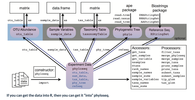
For examining the results of our analysis in R, we primarily be using the Phyloseq package, with some additional packages.
There are many possible file and data types that can be imported into Phyloseq:
To start off, we will load the R libraries we will need
# load the packages
library('phyloseq')
library('tibble')
library('ggplot2')
library('ape')
library('vegan')
We will do the work in the ‘plots’ directory, so in R, set that as the working directory
# set the working directory
setwd('../plots')
Now, we will put together all the elements to create a Phyloseq object
Import the frequency table
First we will import the frequency table.
import_table <- read.table('../otus/otu_frequency_table.tsv',header=TRUE,sep='\t',row.names=1, comment.char = "")
head(import_table)
| AM1 | AM2 | AM3 | AM4 | AM5 | AM6 | AS2 | AS3 | AS4 | AS5 | AS6 | |
|---|---|---|---|---|---|---|---|---|---|---|---|
| <int> | <int> | <int> | <int> | <int> | <int> | <int> | <int> | <int> | <int> | <int> | |
| OTU.1 | 723 | 3634 | 0 | 2907 | 171 | 1956 | 2730 | 2856 | 4192 | 3797 | 3392 |
| OTU.10 | 0 | 0 | 0 | 0 | 0 | 0 | 2223 | 0 | 0 | 1024 | 0 |
| OTU.11 | 1892 | 0 | 0 | 0 | 82 | 113 | 0 | 0 | 0 | 0 | 0 |
| OTU.12 | 0 | 1587 | 0 | 0 | 0 | 0 | 0 | 0 | 0 | 0 | 0 |
| OTU.13 | 0 | 0 | 0 | 0 | 0 | 0 | 0 | 0 | 0 | 1472 | 0 |
| OTU.14 | 0 | 0 | 0 | 0 | 0 | 0 | 0 | 0 | 0 | 0 | 1087 |
Now convert to a matrix for Phyloseq
otumat <- as.matrix(import_table)
head(otumat)
| AM1 | AM2 | AM3 | AM4 | AM5 | AM6 | AS2 | AS3 | AS4 | AS5 | AS6 | |
|---|---|---|---|---|---|---|---|---|---|---|---|
| OTU.1 | 723 | 3634 | 0 | 2907 | 171 | 1956 | 2730 | 2856 | 4192 | 3797 | 3392 |
| OTU.10 | 0 | 0 | 0 | 0 | 0 | 0 | 2223 | 0 | 0 | 1024 | 0 |
| OTU.11 | 1892 | 0 | 0 | 0 | 82 | 113 | 0 | 0 | 0 | 0 | 0 |
| OTU.12 | 0 | 1587 | 0 | 0 | 0 | 0 | 0 | 0 | 0 | 0 | 0 |
| OTU.13 | 0 | 0 | 0 | 0 | 0 | 0 | 0 | 0 | 0 | 1472 | 0 |
| OTU.14 | 0 | 0 | 0 | 0 | 0 | 0 | 0 | 0 | 0 | 0 | 1087 |
Now create an OTU object using the function otu_table
OTU <- otu_table(otumat, taxa_are_rows = TRUE)
head(OTU)
| AM1 | AM2 | AM3 | AM4 | AM5 | AM6 | AS2 | AS3 | AS4 | AS5 | AS6 | |
|---|---|---|---|---|---|---|---|---|---|---|---|
| OTU.1 | 723 | 3634 | 0 | 2907 | 171 | 1956 | 2730 | 2856 | 4192 | 3797 | 3392 |
| OTU.10 | 0 | 0 | 0 | 0 | 0 | 0 | 2223 | 0 | 0 | 1024 | 0 |
| OTU.11 | 1892 | 0 | 0 | 0 | 82 | 113 | 0 | 0 | 0 | 0 | 0 |
| OTU.12 | 0 | 1587 | 0 | 0 | 0 | 0 | 0 | 0 | 0 | 0 | 0 |
| OTU.13 | 0 | 0 | 0 | 0 | 0 | 0 | 0 | 0 | 0 | 1472 | 0 |
| OTU.14 | 0 | 0 | 0 | 0 | 0 | 0 | 0 | 0 | 0 | 0 | 1087 |
Import the taxonomy table
Now we will import the taxonomy table. This is the output from the Sintax analysis.
import_taxa <- read.table('../taxonomy/sintax_taxonomy.tsv',header=TRUE,sep='\t',row.names=1)
head(import_taxa)
| kingdom | phylum | class | order | family | genus | species | Confidence | |
|---|---|---|---|---|---|---|---|---|
| OTU.1 | Eukaryota | Chordata | Actinopteri | Scombriformes | Gempylidae | Thyrsites | Thyrsites_atun | 1.0000000 |
| OTU.2 | Eukaryota | Chordata | Actinopteri | Mugiliformes | Mugilidae | Aldrichetta | Aldrichetta_forsteri | 0.9999999 |
| OTU.3 | Eukaryota | Chordata | Actinopteri | Perciformes | Bovichtidae | Bovichtus | Bovichtus_variegatus | 0.9999979 |
| OTU.4 | Eukaryota | Chordata | Actinopteri | Blenniiformes | Tripterygiidae | Forsterygion | Forsterygion_lapillum | 1.0000000 |
| OTU.5 | Eukaryota | Chordata | Actinopteri | Labriformes | Labridae | Notolabrus | Notolabrus_fucicola | 0.9996494 |
| OTU.6 | Eukaryota | Chordata | Actinopteri | Blenniiformes | Tripterygiidae | Forsterygion | Forsterygion_lapillum | 1.0000000 |
Convert to a matrix:
taxonomy <- as.matrix(import_taxa)
Create a taxonomy class object
TAX <- tax_table(taxonomy)
Import the sample metadata
metadata <- read.table('../docs/sample_metadata.tsv',header = T,sep='\t',row.names = 1)
metadata
| fwd_barcode | rev_barcode | forward_primer | reverse_primer | location | temperature | salinity | sample | |
|---|---|---|---|---|---|---|---|---|
| <chr> | <chr> | <chr> | <chr> | <chr> | <int> | <int> | <chr> | |
| AM1 | GAAGAG | TAGCGTCG | GACCCTATGGAGCTTTAGAC | CGCTGTTATCCCTADRGTAACT | mudflats | 12 | 32 | AM1 |
| AM2 | GAAGAG | TCTACTCG | GACCCTATGGAGCTTTAGAC | CGCTGTTATCCCTADRGTAACT | mudflats | 14 | 32 | AM2 |
| AM3 | GAAGAG | ATGACTCG | GACCCTATGGAGCTTTAGAC | CGCTGTTATCCCTADRGTAACT | mudflats | 12 | 32 | AM3 |
| AM4 | GAAGAG | ATCTATCG | GACCCTATGGAGCTTTAGAC | CGCTGTTATCCCTADRGTAACT | mudflats | 10 | 32 | AM4 |
| AM5 | GAAGAG | ACAGATCG | GACCCTATGGAGCTTTAGAC | CGCTGTTATCCCTADRGTAACT | mudflats | 12 | 34 | AM5 |
| AM6 | GAAGAG | ATACTGCG | GACCCTATGGAGCTTTAGAC | CGCTGTTATCCCTADRGTAACT | mudflats | 10 | 34 | AM6 |
| AS2 | GAAGAG | AGATACTC | GACCCTATGGAGCTTTAGAC | CGCTGTTATCCCTADRGTAACT | shore | 12 | 32 | AS2 |
| AS3 | GAAGAG | ATGCGATG | GACCCTATGGAGCTTTAGAC | CGCTGTTATCCCTADRGTAACT | shore | 12 | 32 | AS3 |
| AS4 | GAAGAG | TGCTACTC | GACCCTATGGAGCTTTAGAC | CGCTGTTATCCCTADRGTAACT | shore | 10 | 34 | AS4 |
| AS5 | GAAGAG | ACGTCATG | GACCCTATGGAGCTTTAGAC | CGCTGTTATCCCTADRGTAACT | shore | 14 | 34 | AS5 |
| AS6 | GAAGAG | TCATGTCG | GACCCTATGGAGCTTTAGAC | CGCTGTTATCCCTADRGTAACT | shore | 10 | 34 | AS6 |
| ASN | GAAGAG | AGACGCTC | GACCCTATGGAGCTTTAGAC | CGCTGTTATCCCTADRGTAACT | negative | NA | NA | ASN |
As we are not using the negative control, we will remove it
metadata <- metadata[1:11,1:8]
tail(metadata)
| fwd_barcode | rev_barcode | forward_primer | reverse_primer | location | temperature | salinity | sample | |
|---|---|---|---|---|---|---|---|---|
| <chr> | <chr> | <chr> | <chr> | <chr> | <int> | <int> | <chr> | |
| AM6 | GAAGAG | ATACTGCG | GACCCTATGGAGCTTTAGAC | CGCTGTTATCCCTADRGTAACT | mudflats | 10 | 34 | AM6 |
| AS2 | GAAGAG | AGATACTC | GACCCTATGGAGCTTTAGAC | CGCTGTTATCCCTADRGTAACT | shore | 12 | 32 | AS2 |
| AS3 | GAAGAG | ATGCGATG | GACCCTATGGAGCTTTAGAC | CGCTGTTATCCCTADRGTAACT | shore | 12 | 32 | AS3 |
| AS4 | GAAGAG | TGCTACTC | GACCCTATGGAGCTTTAGAC | CGCTGTTATCCCTADRGTAACT | shore | 10 | 34 | AS4 |
| AS5 | GAAGAG | ACGTCATG | GACCCTATGGAGCTTTAGAC | CGCTGTTATCCCTADRGTAACT | shore | 14 | 34 | AS5 |
| AS6 | GAAGAG | TCATGTCG | GACCCTATGGAGCTTTAGAC | CGCTGTTATCCCTADRGTAACT | shore | 10 | 34 | AS6 |
Create a Phyloseq sample_data-class
META <- sample_data(metadata)
Create a Phyloseq object
Now that we have all the components, it is time to create a Phyloseq object
physeq <- phyloseq(OTU,TAX,META)
physeq
    phyloseq-class experiment-level object
    otu_table()   OTU Table:         [ 33 taxa and 11 samples ]
    sample_data() Sample Data:       [ 11 samples by 8 sample variables ]
    tax_table()   Taxonomy Table:    [ 33 taxa by 8 taxonomic ranks ]
One last thing we will do is to convert two of the metadata variables from continuous to ordinal. This will help us graph these fields later
sample_data(physeq)$temperature <- as(sample_data(physeq)$temperature, "character")

sample_data(physeq)$salinity <- as(sample_data(physeq)$salinity, "character")
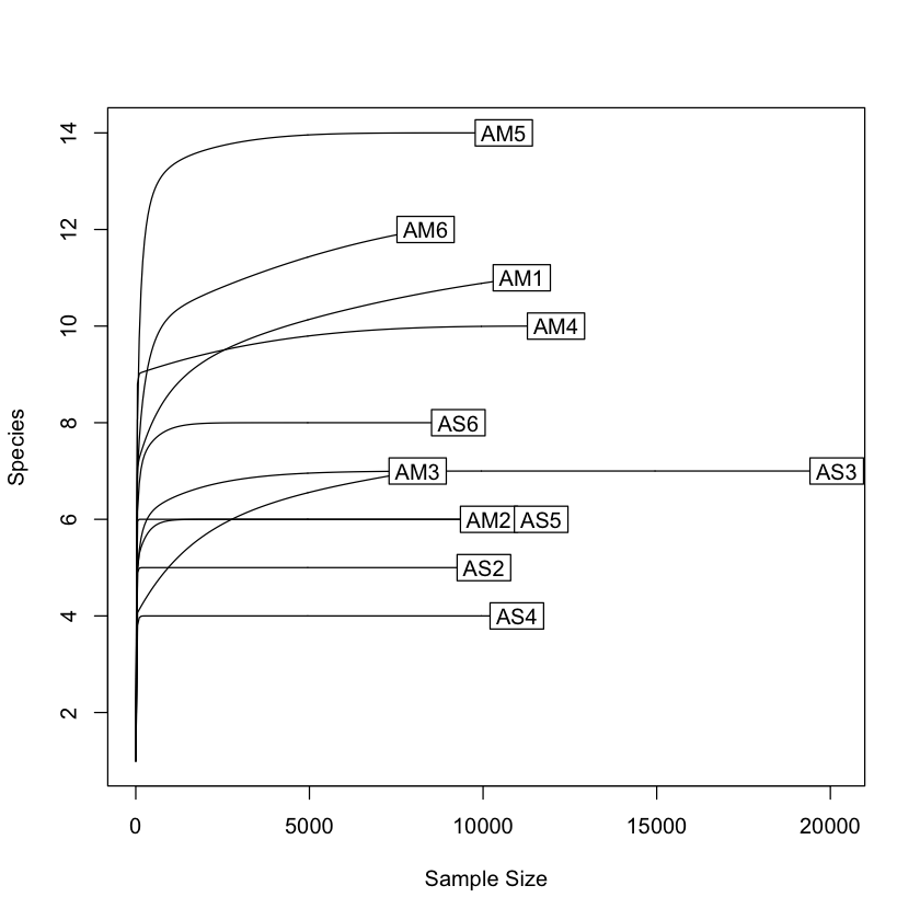
Initial data inspection
Now that we have our Phyloseq object, we will take a look at it. One of the first steps is to check alpha rarefaction of species richness. This is done to show that there has been sufficient sequencing to detect most species (OTUs).
rarecurve(t(otu_table(physeq)), step=50, cex=1)
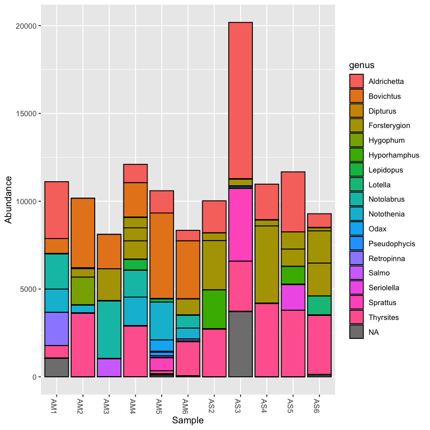
create a bar plot of abundance
plot_bar(physeq)
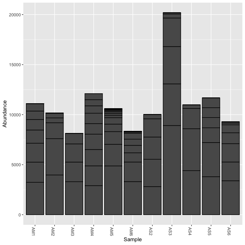
print(min(sample_sums(physeq)))
print(max(sample_sums(physeq)))
    [1] 8117
    [1] 20184
Rarefy the data
From the initial look at the data, it is obvious that the sample AS3 has about twice as many reads as any of the other samples. We can use rarefaction to simulate an even number of reads per sample. Rarefying the data is preferred for some analyses, though there is some debate. We will create a rarefied version of the Phyloseq object.
we will rarefy the data around 90% of the lowest sample
physeq.rarefied <- rarefy_even_depth(physeq, rngseed=1, sample.size=0.9*min(sample_sums(physeq)), replace=F)
    `set.seed(1)` was used to initialize repeatable random subsampling.

    Please record this for your records so others can reproduce.

    Try `set.seed(1); .Random.seed` for the full vector

    ...
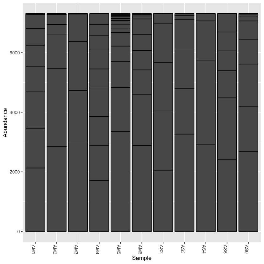
now plot the rarefied version
plot_bar(physeq.rarefied)
Saving your work to files
You can save the Phyloseq object you just created, and then import it into another R session later. This way you do not have to re-import all the components separately.
Also, below are a couple of examples of saving graphs. There are many options for this that you can explore to create publication-quality graphics of your results
Save the phyloseq object
saveRDS(physeq, 'fish_phyloseq.rds')
Also save the rarefied version
saveRDS(physeq.rarefied, 'fish_phyloseq_rarefied.rds')
To later read the Phyloseq object into your R session:
first the original
physeq <- readRDS('fish_phyloseq.rds')
print(physeq)
Saving a graph to file
# open a pdf file
pdf('species_richness_plot.pdf')
# run the plot, or add the saved one
rarecurve(t(otu_table(physeq)), step=50, cex=1.5, col='blue',lty=2)
# close the pdf
dev.off()
pdf: 2
there are other graphic formats that you can use
jpeg("species_richness_plot.jpg", width = 800, height = 800)
rarecurve(t(otu_table(physeq)), step=50, cex=1.5, col='blue',lty=2)
dev.off()
pdf: 2
Key Points
Phyloseq has many functions to explore metabarcoding data
Results from early lessons must be converted to a matrix
Phyloseq is integrated with ggplot to expand graphic output
Statistics and Graphing with R
Overview
Teaching: 10 min
Exercises: 50 minQuestions
How do I use ggplot and other programs with Phyloseq?
What statistical approaches do I use to explore my metabarcoding results?
Objectives
Create bar plots of taxonomy and use them to show differences across the metadata
Create distance ordinations and use them to make PCoA plots
Make subsets of the data to explore specific aspects of your results
In this lesson there are several examples for plotting the results of your analysis. As mentioned in the previous lesson, here are some links with additional graphing examples:
-
The Phyloseq web page has many good tutorials
-
The Micca pipeline has a good intro tutorial for Phyloseq
-
Remember, if you are starting a new notebook, to set the working directory and read in the Phyloseq object:
setwd(../plots)
# load the packages
library('phyloseq')
library('tibble')
library('ggplot2')
library('ape')
library('vegan')

physeq <- readRDS('fish_phyloseq.rds')
print(physeq)
Plotting taxonomy
Using the plot_bar function, we can plot the relative abundance of taxa across samples
plot_bar(physeq, fill='genus')
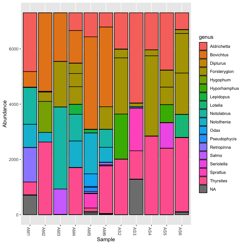
Plotting the taxonomy with the rarefied dataset can help to compare abundance across samples
plot_bar(physeq.rarefied, fill='genus')
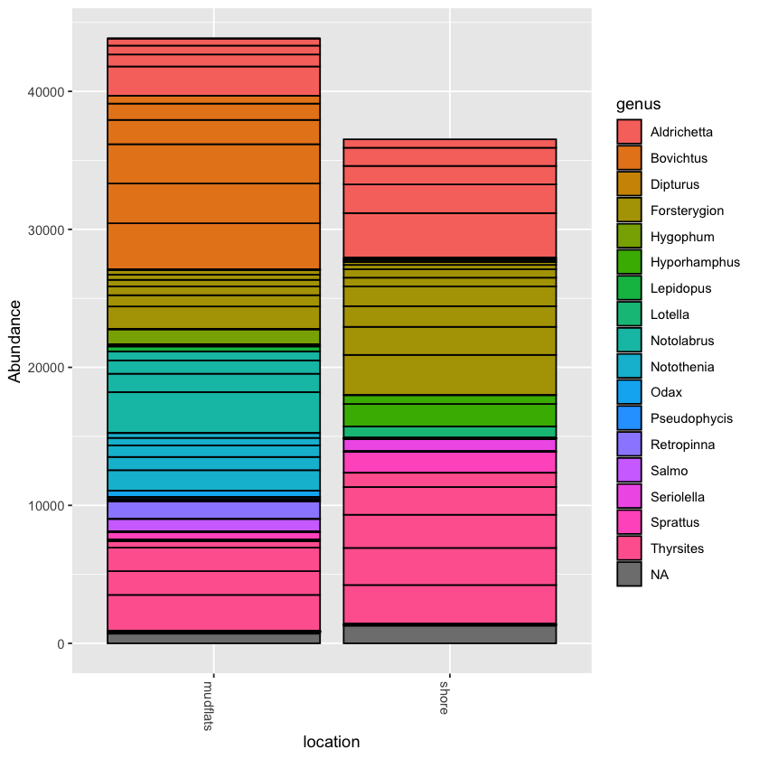
You can collapse the frequency counts across metadata categories, such as location
plot_bar(physeq.rarefied, x='location', fill='genus')
Exercise: collapse counts around temperature
Try to collapse counts around another metadata category, like temperature. Then try filling at a different taxonomic level, like order or family
Solution
plot_bar(physeq.rarefied, x='temperature', fill='family')
Incorporate ggplot into your Phyloseq graph
Now we will try to add ggplot elements to the graph
Add ggplot facet_wrap tool to graph
Try using facet_wrap to break your plot into separate parts
Hint: First save your plot to a variable, then you can add to it
Solution
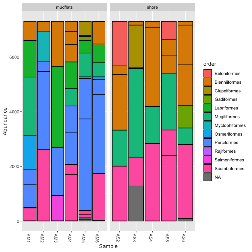
barplot1 <- plot_bar(physeq.rarefied, fill='order')

barplot1 + facet_wrap(~location, scales="free_x",nrow=1)
Combine visuals to present more information
Now that you can use facet_wrap, try to show both location and temperature in a single graph.
Hint: Try to combine from the above two techniques
Solution
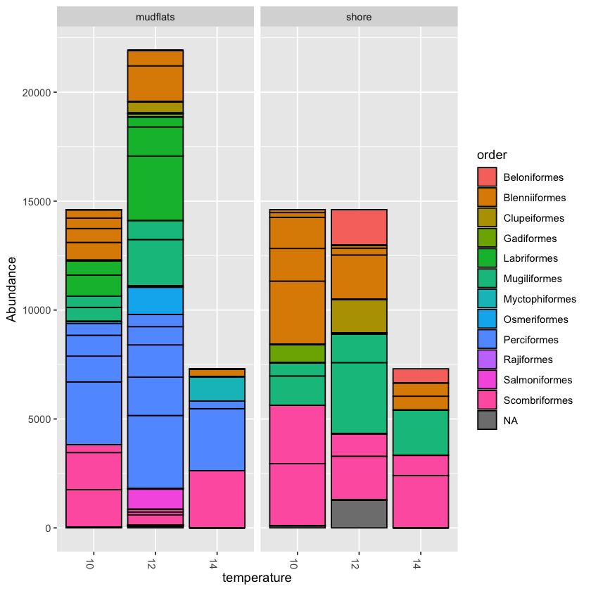
barplot2 <- plot_bar(physeq.rarefied, x="temperature", fill='order') +
facet_wrap(~location, scales="free_x", nrow=1)

barplot2
Community ecology
The Phyloseq package has many functions for exploring diversity within and between samples. This includes multiple methods of calculating distance matrices between samples.
An ongoing debate with metabarcoding data is whether relative frequency of OTUs should be taken into account, or whether they should be scored as presence or absence. Phyloseq allows you to calculate distance using both qualitative (i.e. presence/absence) and quantitative (abundance included) measures, taken from community ecology diversity statistics.
For qualitative distance use the Jaccard method
jac_dist <- distance(physeq.rarefied, method = "jaccard", binary = TRUE)
jac_dist
jac_dist
              AM1       AM2       AM3       AM4       AM5       AM6       AS2
    AM2 0.7692308
    AM3 0.6923077 0.8181818
    AM4 0.5714286 0.6666667 0.7857143
    AM5 0.6666667 0.8235294 0.7647059 0.6666667
    AM6 0.4285714 0.8000000 0.7333333 0.6250000 0.5555556
    AS2 0.8461538 0.7777778 0.9090909 0.7500000 0.8823529 0.8666667
    AS3 0.8666667 0.8181818 0.9230769 0.8666667 0.7647059 0.8823529 0.6666667
    AS4 0.8333333 0.7500000 0.9000000 0.7272727 0.8750000 0.8571429 0.2000000
    AS5 0.8571429 0.8000000 0.9166667 0.7692308 0.8888889 0.8750000 0.1666667
    AS6 0.8750000 0.8333333 0.9285714 0.8000000 0.9000000 0.8888889 0.5555556
              AS3       AS4       AS5
    AM2
    AM3
    AM4
    AM5
    AM6
    AS2
    AS3
    AS4 0.6250000
    AS5 0.7000000 0.3333333
    AS6 0.7500000 0.5000000 0.6000000
Now you can run the ordination function in Phyloseq and then plot it.
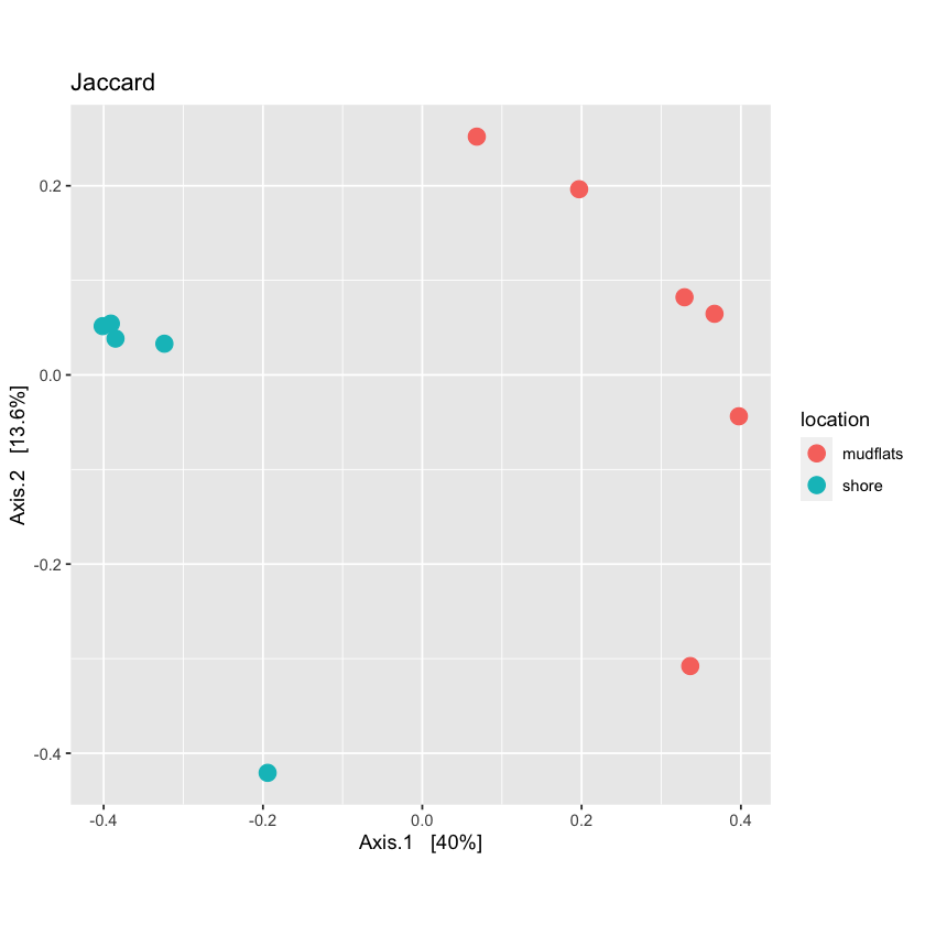
qual_ord <- ordinate(physeq.rarefied, method="PCoA", distance=jac_dist)
plot_jac <- plot_ordination(physeq.rarefied, qual_ord, color="location", title='Jaccard') + theme(aspect.ratio=1) + geom_point(size=4)
plot_jac
Using quantitative distances
For quantitative distance use the Bray-Curtis method:
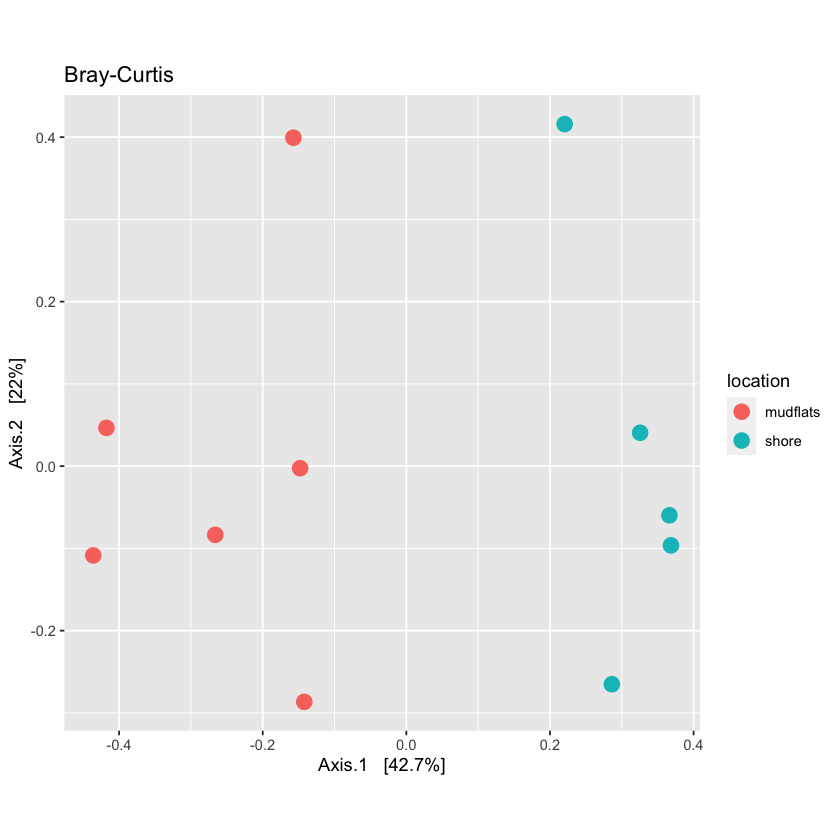
bc_dist <- distance(physeq.rarefied, method = "bray", binary = FALSE)
Now run ordination on the quantitative distances and plot them
Also try to make the points of the graph smaller
Solution
quant_ord <- ordinate(physeq.rarefied, method="PCoA", distance=bc_dist)plot_bc <- plot_ordination(physeq.rarefied, quant_ord, color="location", title='Bray-Curtis') + theme(aspect.ratio=1) + geom_point(size=3) plot_bc
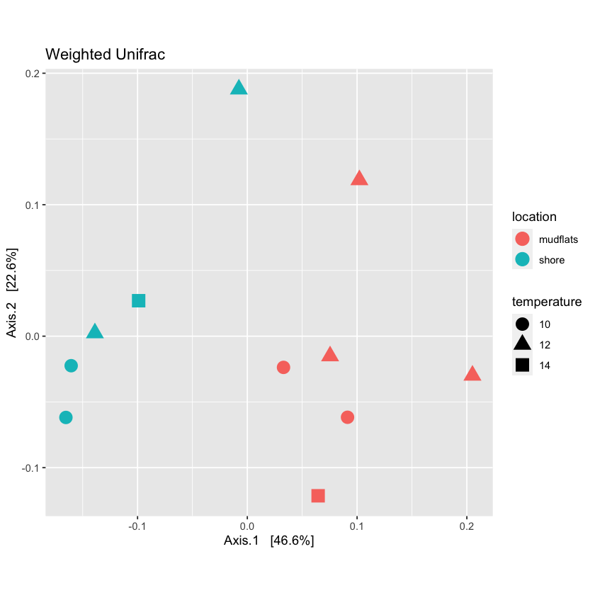
View multiple variables on a PCoA plot
Phyloseq allows you to graph multiple characteristics. Try to plot location by color and temperature by shape
Solution
plot_locTemp <- plot_ordination(physeq.rarefied, quant_ord, color="location", shape='temperature', title="Jaccard Location and Temperature") +
theme(aspect.ratio=1) +
geom_point(size=4)

plot_locTemp
Permutational ANOVA
Phyloseq includes the adonis function to run a PERMANOVA to determine if OTUs from specific metadata fields are significantly different from each other.
adonis(bc_dist ~ sample_data(physeq.rarefied)$location)
    Call:
    adonis(formula = bc_dist ~ sample_data(physeq.rarefied)$location)

    Permutation: free
    Number of permutations: 999

    Terms added sequentially (first to last)

                                          Df SumsOfSqs  MeanSqs F.Model      R2
    sample_data(physeq.rarefied)$location  1   0.13144 0.131438   5.938 0.39751
    Residuals                              9   0.19921 0.022135         0.60249
    Total                                 10   0.33065                  1.00000
                                          Pr(>F)
    sample_data(physeq.rarefied)$location  0.002 **
    Residuals
    Total
    ---
    Signif. codes:  0 ‘***’ 0.001 ‘**’ 0.01 ‘*’ 0.05 ‘.’ 0.1 ‘ ’ 1
Is temperature significantly different?
Run PERMANOVA on the temperature variable
Solution
adonis(bc_dist ~ sample_data(physeq.rarefied)$temperature)Call: adonis(formula = bc_dist ~ sample_data(physeq.rarefied)$temperature) Permutation: free Number of permutations: 999 Terms added sequentially (first to last) Df SumsOfSqs MeanSqs F.Model R2 sample_data(physeq.rarefied)$temperature 2 0.06606 0.033031 0.99869 0.19979 Residuals 8 0.26459 0.033074 0.80021 Total 10 0.33065 1.00000 Pr(>F) sample_data(physeq.rarefied)$temperature 0.441 Residuals TotalTemperature is not significantly different across samples
Subsetting data
It is possible to take subsets of the Phyloseq object you have created. You can subset by taxa or samples.
Subsetting by taxonomy
Often there are so many taxonomic groups represented, that it is useful to create a subset of the data that contains only OTUs belonging to a taxonomic rank. This is done with the subset_taxa function. In the example dataset provided, there are not too many taxa included, but for larger datasets this can be very useful
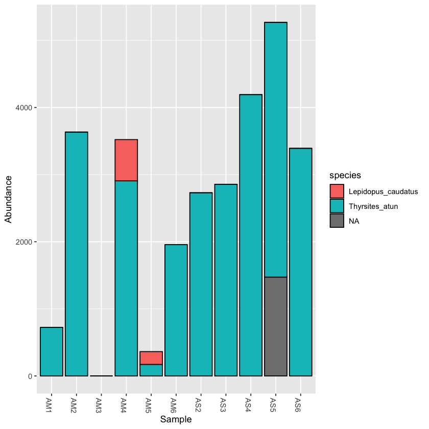
scomb <- subset_taxa(physeq, order=='Scombriformes')
the subsetted database is still a valid Phyloseq object:
scomb
    phyloseq-class experiment-level object
    otu_table()   OTU Table:         [ 3 taxa and 11 samples ]
    sample_data() Sample Data:       [ 11 samples by 8 sample variables ]
    tax_table()   Taxonomy Table:    [ 3 taxa by 8 taxonomic ranks ]
plot_bar(scomb, fill='species')
Exercise: take a subset of a taxon and plot it
Subset samples
Now we will try to make a subset of the Phyloseq object based on a field from the sample metadata table.
First, let’s look at the metadata:
sample_data(physeq)
| fwd_barcode | rev_barcode | forward_primer | reverse_primer | location | temperature | salinity | sample | |
|---|---|---|---|---|---|---|---|---|
| <chr> | <chr> | <chr> | <chr> | <chr> | <fct> | <fct> | <chr> | |
| AM1 | GAAGAG | TAGCGTCG | GACCCTATGGAGCTTTAGAC | CGCTGTTATCCCTADRGTAACT | mudflats | 12 | 32 | AM1 |
| AM2 | GAAGAG | TCTACTCG | GACCCTATGGAGCTTTAGAC | CGCTGTTATCCCTADRGTAACT | mudflats | 14 | 32 | AM2 |
| AM3 | GAAGAG | ATGACTCG | GACCCTATGGAGCTTTAGAC | CGCTGTTATCCCTADRGTAACT | mudflats | 12 | 32 | AM3 |
| AM4 | GAAGAG | ATCTATCG | GACCCTATGGAGCTTTAGAC | CGCTGTTATCCCTADRGTAACT | mudflats | 10 | 32 | AM4 |
| AM5 | GAAGAG | ACAGATCG | GACCCTATGGAGCTTTAGAC | CGCTGTTATCCCTADRGTAACT | mudflats | 12 | 34 | AM5 |
| AM6 | GAAGAG | ATACTGCG | GACCCTATGGAGCTTTAGAC | CGCTGTTATCCCTADRGTAACT | mudflats | 10 | 34 | AM6 |
| AS2 | GAAGAG | AGATACTC | GACCCTATGGAGCTTTAGAC | CGCTGTTATCCCTADRGTAACT | shore | 12 | 32 | AS2 |
| AS3 | GAAGAG | ATGCGATG | GACCCTATGGAGCTTTAGAC | CGCTGTTATCCCTADRGTAACT | shore | 12 | 32 | AS3 |
| AS4 | GAAGAG | TGCTACTC | GACCCTATGGAGCTTTAGAC | CGCTGTTATCCCTADRGTAACT | shore | 10 | 34 | AS4 |
| AS5 | GAAGAG | ACGTCATG | GACCCTATGGAGCTTTAGAC | CGCTGTTATCCCTADRGTAACT | shore | 14 | 34 | AS5 |
| AS6 | GAAGAG | TCATGTCG | GACCCTATGGAGCTTTAGAC | CGCTGTTATCCCTADRGTAACT | shore | 10 | 34 | AS6 |
The command is similar to the subset_taxa command. For example, if we want to only analyse the samples found in the mudflats:
mud <- subset_samples(physeq, location=='mudflats')

mud
The output is still a Phyloseq object:
    phyloseq-class experiment-level object
    otu_table()   OTU Table:         [ 33 taxa and 6 samples ]
    sample_data() Sample Data:       [ 6 samples by 8 sample variables ]
    tax_table()   Taxonomy Table:    [ 33 taxa by 8 taxonomic ranks ]
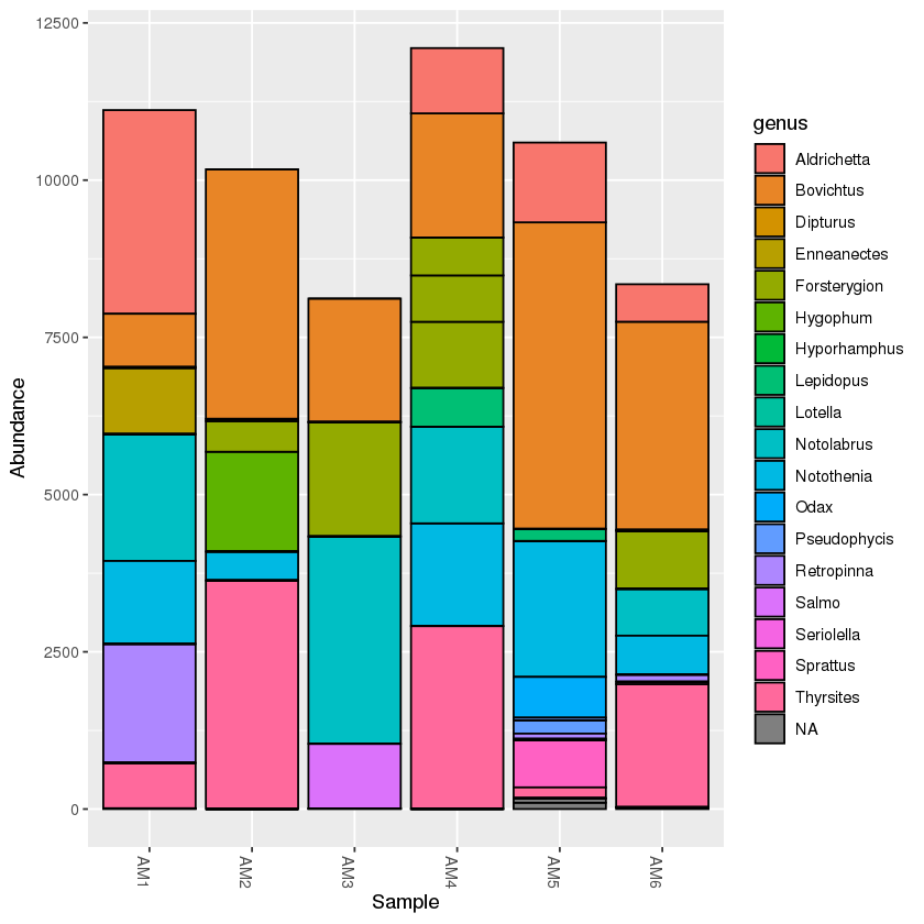
A taxonomy bar plot will only show the mudflats samples:
plot_bar(mud, fill='genus')
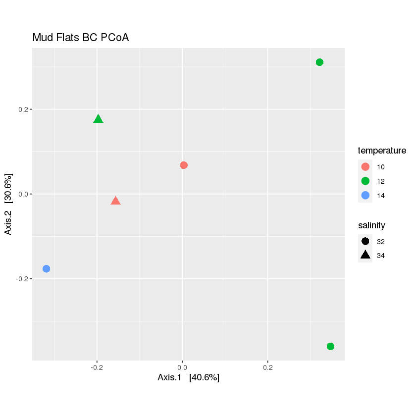
Exercise: create a PCoA plot of the mudflats subset
Hint: is there anything that should be done with the data before plotting?
Solution
First, rarefy the new dataset:
mud.rarefied <- rarefy_even_depth(mud, rngseed=1, sample.size=0.9*min(sample_sums(mud)), replace=F)Now, calculate the distance and ordination
mud_dist <- distance(mud.rarefied, method = 'bray', binary=FALSE)

mud_ord <- ordinate(mud.rarefied, method="PCoA", distance=mud_dist)
Finally, plot the ordination
plot_mud <- plot_ordination(mud.rarefied, mud_ord, color='temperature',shape='salinity', title="Mud Flats BC PCoA")+
theme(aspect.ratio=1)+ geom_point(size=4)

plot_mud
Merge OTUs by taxa
The final function we will present is to merge the OTUs by taxonomy. You will notice that there are often multiple OTUs that are assigned to a single species or genus. This can be due to multiple factors, such as sequence error, gaps in the reference database, or a species that varies in the target region. If you are interested in focusing on the taxonomy, then it is useful to merge OTUs that assign to the same taxon. Fortunately, Phyloseq provides a useful function to do this.
We will merge all OTUs at the lowest taxonomic level
phyMerge <- tax_glom(physeq, taxrank = 'species',NArm = T)
Now have a look at the taxonomy table. You should see that there are fewer OTUs.
tax_table(phyMerge)
| kingdom | phylum | class | order | family | genus | species | Confidence | |
|---|---|---|---|---|---|---|---|---|
| OTU.8 | Eukaryota | Chordata | Actinopteri | Clupeiformes | Clupeidae | Sprattus | Sprattus_muelleri | NA |
| OTU.21 | Eukaryota | Chordata | Actinopteri | Clupeiformes | Clupeidae | Sprattus | Sprattus_antipodum | NA |
| OTU.17 | Eukaryota | Chordata | Actinopteri | Blenniiformes | Tripterygiidae | Enneanectes | Enneanectes_carminalis | NA |
| OTU.4 | Eukaryota | Chordata | Actinopteri | Blenniiformes | Tripterygiidae | Forsterygion | Forsterygion_lapillum | NA |
| OTU.11 | Eukaryota | Chordata | Actinopteri | Osmeriformes | Retropinnidae | Retropinna | Retropinna_retropinna | NA |
| OTU.10 | Eukaryota | Chordata | Actinopteri | Beloniformes | Hemiramphidae | Hyporhamphus | Hyporhamphus_melanochir | NA |
| OTU.3 | Eukaryota | Chordata | Actinopteri | Perciformes | Bovichtidae | Bovichtus | Bovichtus_variegatus | NA |
| OTU.7 | Eukaryota | Chordata | Actinopteri | Perciformes | Nototheniidae | Notothenia | Notothenia_angustata | NA |
| OTU.2 | Eukaryota | Chordata | Actinopteri | Mugiliformes | Mugilidae | Aldrichetta | Aldrichetta_forsteri | NA |
| OTU.5 | Eukaryota | Chordata | Actinopteri | Labriformes | Labridae | Notolabrus | Notolabrus_fucicola | NA |
| OTU.22 | Eukaryota | Chordata | Actinopteri | Labriformes | Odacidae | Odax | Odax_pullus | NA |
| OTU.14 | Eukaryota | Chordata | Actinopteri | Gadiformes | Moridae | Lotella | Lotella_rhacina | NA |
| OTU.23 | Eukaryota | Chordata | Actinopteri | Gadiformes | Moridae | Pseudophycis | Pseudophycis_barbata | NA |
| OTU.19 | Eukaryota | Chordata | Actinopteri | Scombriformes | Trichiuridae | Lepidopus | Lepidopus_caudatus | NA |
| OTU.1 | Eukaryota | Chordata | Actinopteri | Scombriformes | Gempylidae | Thyrsites | Thyrsites_atun | NA |
| OTU.12 | Eukaryota | Chordata | Actinopteri | Myctophiformes | Myctophidae | Hygophum | Hygophum_hanseni | NA |
Exercise
In the previous example, you might have noticed that any OTU that was not resolved to species (i.e. ‘NA’ in the species column) was removed from the table. Try to rerun the function, keeping all the unresolved species.
Solution
phyMergeNA <- tax_glom(physeq, taxrank = 'species',NArm = F)tax_table(phyMergeNA)
A taxonomyTable: 23 × 8 of type chr kingdom phylum class order family genus species Confidence OTU.33 Eukaryota Chordata NA NA NA NA NA NA OTU.8 Eukaryota Chordata Actinopteri Clupeiformes Clupeidae Sprattus Sprattus_muelleri NA OTU.21 Eukaryota Chordata Actinopteri Clupeiformes Clupeidae Sprattus Sprattus_antipodum NA OTU.29 Eukaryota Chordata Actinopteri Clupeiformes Clupeidae Sprattus NA NA OTU.17 Eukaryota Chordata Actinopteri Blenniiformes Tripterygiidae Enneanectes Enneanectes_carminalis NA OTU.4 Eukaryota Chordata Actinopteri Blenniiformes Tripterygiidae Forsterygion Forsterygion_lapillum NA OTU.11 Eukaryota Chordata Actinopteri Osmeriformes Retropinnidae Retropinna Retropinna_retropinna NA OTU.15 Eukaryota Chordata Actinopteri Salmoniformes Salmonidae Salmo NA NA OTU.10 Eukaryota Chordata Actinopteri Beloniformes Hemiramphidae Hyporhamphus Hyporhamphus_melanochir NA OTU.3 Eukaryota Chordata Actinopteri Perciformes Bovichtidae Bovichtus Bovichtus_variegatus NA OTU.7 Eukaryota Chordata Actinopteri Perciformes Nototheniidae Notothenia Notothenia_angustata NA OTU.2 Eukaryota Chordata Actinopteri Mugiliformes Mugilidae Aldrichetta Aldrichetta_forsteri NA OTU.9 Eukaryota Chordata Actinopteri NA NA NA NA NA OTU.5 Eukaryota Chordata Actinopteri Labriformes Labridae Notolabrus Notolabrus_fucicola NA OTU.22 Eukaryota Chordata Actinopteri Labriformes Odacidae Odax Odax_pullus NA OTU.31 Eukaryota Chordata Chondrichthyes Rajiformes Rajidae Dipturus NA NA OTU.14 Eukaryota Chordata Actinopteri Gadiformes Moridae Lotella Lotella_rhacina NA OTU.23 Eukaryota Chordata Actinopteri Gadiformes Moridae Pseudophycis Pseudophycis_barbata NA OTU.28 Eukaryota Chordata Actinopteri Gadiformes Moridae Pseudophycis NA NA OTU.19 Eukaryota Chordata Actinopteri Scombriformes Trichiuridae Lepidopus Lepidopus_caudatus NA OTU.1 Eukaryota Chordata Actinopteri Scombriformes Gempylidae Thyrsites Thyrsites_atun NA OTU.13 Eukaryota Chordata Actinopteri Scombriformes Centrolophidae Seriolella NA NA OTU.12 Eukaryota Chordata Actinopteri Myctophiformes Myctophidae Hygophum Hygophum_hanseni NA
Exercise
What would happen if you set the
taxrankparameter in thetax_glomfunction to a higher taxonomic level, like family?Solution
phyMergeFAM <- tax_glom(physeq, taxrank = 'family',NArm = T)

tax_table(phyMergeFAM)
A taxonomyTable: 16 × 8 of type chr kingdom phylum class order family genus species Confidence OTU.8 Eukaryota Chordata Actinopteri Clupeiformes Clupeidae NA NA NA OTU.4 Eukaryota Chordata Actinopteri Blenniiformes Tripterygiidae NA NA NA OTU.11 Eukaryota Chordata Actinopteri Osmeriformes Retropinnidae NA NA NA OTU.15 Eukaryota Chordata Actinopteri Salmoniformes Salmonidae NA NA NA OTU.10 Eukaryota Chordata Actinopteri Beloniformes Hemiramphidae NA NA NA OTU.3 Eukaryota Chordata Actinopteri Perciformes Bovichtidae NA NA NA OTU.7 Eukaryota Chordata Actinopteri Perciformes Nototheniidae NA NA NA OTU.2 Eukaryota Chordata Actinopteri Mugiliformes Mugilidae NA NA NA OTU.5 Eukaryota Chordata Actinopteri Labriformes Labridae NA NA NA OTU.22 Eukaryota Chordata Actinopteri Labriformes Odacidae NA NA NA OTU.31 Eukaryota Chordata Chondrichthyes Rajiformes Rajidae NA NA NA OTU.14 Eukaryota Chordata Actinopteri Gadiformes Moridae NA NA NA OTU.19 Eukaryota Chordata Actinopteri Scombriformes Trichiuridae NA NA NA OTU.1 Eukaryota Chordata Actinopteri Scombriformes Gempylidae NA NA NA OTU.13 Eukaryota Chordata Actinopteri Scombriformes Centrolophidae NA NA NA OTU.12 Eukaryota Chordata Actinopteri Myctophiformes Myctophidae NA NA NA
Key Points
The Phyloseq package has many useful features to conduct statistical analyses of your data
Introduction to Qiime
Overview
Teaching: 10 min
Exercises: 5 minQuestions
How do I import today’s results into Qiime?
Objectives
Identify the main components of metabarcoding and how to integrate them into a Qiime workflow
Overview
The Qiime2 package is an open-source system that incorporates multiple, stand-alone programs, giving you many options to run your analysis. The different programs are provided as plug-ins to provide maximum flexibility. The Qiime2 docs webpage has all the information you need to get started on processing metabarcoding data. There are multiple tutorials available, including a detailed overview of the available plugins and links to the concepts involved.
It is possible to run the entirety of your analysis within the Qiime2 system, but today we will just show how to import the results of the earlier lessons into the Qiime format, and then you will be able to follow most of the tutorials on the website.
First, here is a quick guided tour of the system.
Here is an overview of the Qiime2 workflow:
One of the main concepts of using Qiime is that all data is represented by what they refer to as “artifacts”, which are actually compressed folders that contain the data and metadata about the data. This is done so that all data files are tracked and logged through the system. In order to use Qiime data must be imported into their system; as well, to use the outputs of Qiime in other programs they must be exported (though some visuals provide a way to download flat files of some outputs).
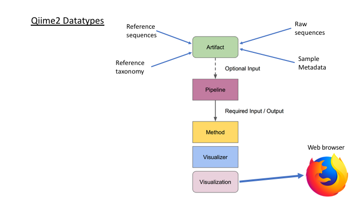
Often you do not want to start at the beginning or finish at the end of a pipeline. Once you are able to import today’s results, you will be able to start where you wish.
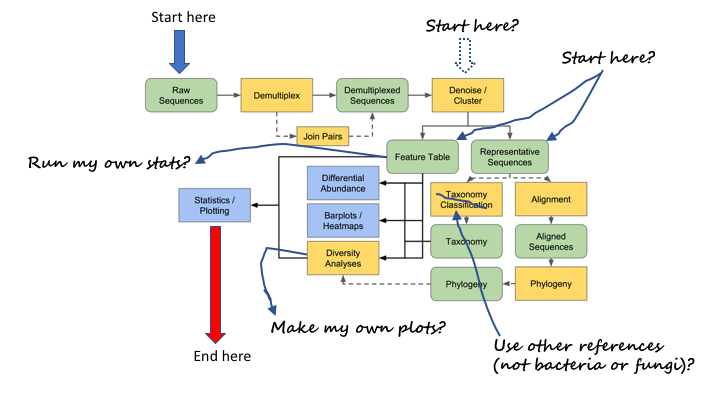
Tour of Qiime2 website
Here is a link to the resources on the Qiime2 website
Getting started: importing files into Qiime2 format
In the command line, we will first load the Qiime2 module:
$ module purge
$ module load QIIME2/2021.4
To see the options for any Qiime2 command, you can use help:
$ qiime tools import --help
There are just a few arguments for importing files, but many possible types and formats. Two of the commands are sort of help commands in that they show what is possible to import.
We can view those by just entering the option:
$ qiime tools import --show-importable-types
Sometimes it is necessary to specify the format of the input file. We can view those as well:
$ qiime tools import --show-importable-formats
These two arguments provide a good guide when you are trying to figure out the kind of file you are importing
Importing OTU fasta file and frequency table
To import the outputs of the Denoising and clustering lesson
module load QIIME2/2021.4
The Qiime import command (substitute the name of your otu file):
qiime tools import \
  --type 'FeatureData[Sequence]' \
  --input-path otus.fasta  \
  --output-path otus.qza
If the command/script worked then you should have a file called otus.qza in your /otus folder. All Qiime artifacts end in .qza, and all visuals end in .qzv.
We cannot import the frequency table directly into Qiime. First we have to convert our table into the biom format. Then the biom format will be imported to Qiime. Create a script called import_freq_table_to_qiime.sh and then put these commands:
biom convert -i otu_frequency_table.tsv \
 -o fish_frequency.biom \
 --to-hdf5

qiime tools import \
  --input-path fish_frequency.biom \
  --type 'FeatureTable[Frequency]' \
  --input-format BIOMV210Format \
  --output-path otu_frequency_table.qza
The output of this script should be two files: a .biom file and a qiime .qza frequency table file.
Importing taxonomy files into Qiime
import taxonomy output (with converter script)
Qiime has several methods to assign taxonomy to your OTUs (see Lesson 4). In order to run these, you must first convert the reference database to a Qiime flat file format, and then import it to Qiime. For the first part, you can use the tax_format tool in the Crabs program. If you have not done so, run the command to convert the reference file.
crabs_v1.0.1 tax_format \
  --input ref_fasta.fasta \
  --output ref_qiime \
  --format qiif
You will notice that Crabs has split the original file into two separate files. One of these is a fasta file with the sequences and sequence ID, and the other is a table that has the taxonomic lineage for each sequence ID. Now you can import each of these files into Qiime.
qiime tools import \
  --type 'FeatureData[Sequence]' \
  --input-path qiime_ref.fasta \
  --output-path qiime.refseqs.qza

qiime tools import \
  --type 'FeatureData[Taxonomy]' \
  --input-format HeaderlessTSVTaxonomyFormat \
  --input-path qiime_ref.taxon \
  --output-path qiime.taxon.qza
Now you are ready to assign taxonomy using either the BLAST or VSEARCH methods (see below). If you would like to run the Naive Bayes method, there is one further step, which is to train the sequences using a machine learning algorithm. However, as this takes time, one has been prepared for this course: lrRNA_fish_db_classifier.qza
For future reference, here is an example training command:
qiime feature-classifier fit-classifier-naive-bayes \
  --i-reference-reads otus.qza \
  --i-reference-taxonomy qiime.taxon.qza \
  --o-classifier lrRNA_fish_db_classifier.qza \
  --verbose
Using your imported files in Qiime
Now that you have all your outputs in Qiime format, you can use them for most of the tutorials on the Qiime web page.
Taxonomy assignment with Qiime
You can run three different methods in Qiime to do taxonomy assignment. For one example, see the basic taxonomic analysis tutorial. Below are examples for each of the methods, indicating which of our imported files to use.
BLAST Taxonomy Assignment
qiime feature-classifier classify-consensus-blast \
  --i-query otus.qza \
  --i-reference-reads qiime.refseqs.qza \
  --i-reference-taxonomy qiime.taxon.qza \
  --o-classification blast_output_taxonomy.qza \
  --verbose
See the classify-consensus-blast plugin page for explanation of parameters and additional options
VSEARCH Taxonomy Assignment
qiime feature-classifier classify-consensus-vsearch \
  --i-query otus.qza \
  --i-reference-reads qiime.refseqs.qza \
  --i-reference-taxonomy qiime.taxon.qza \
  --o-classification vsearch_output_taxonomy.qza \
  --verbose
See the classify-consensus-vsearch plugin page for explanation of parameters and additional options
Naive Bayes Taxonomy Assignment
qiime feature-classifier classify-sklearn \
  --i-reads otus.qza \
  --i-classifier lrRNA_fish_db_classifier.qza \
  --o-classification nb_output_taxonomy.qza \
  --verbose
See the classify-sklearn plugin page for explanation of parameters and additional options
Diversity analyses with Qiime
There are many analyses included in Qiime for doing community ecology statistics, including alpha and beta diversity. You can see an example in the Alpha and beta diversity analysis tutorial.
The main files that are used for most of Qiime’s diversity analyses are the frequency table and the sample metadata file. So, once you have imported the frequency table you can run many analyses (the sample metadata file is one of the few in the Qiime multiverse that remains in flat file format). Qiime has a pipeline command that will run multiple alpha and beta diversity metrics in one go, outputting everything to a separate folder.
The only other statistic that you will need for this is the sampling depth, which is the number that was used for rarefaction in Lesson 06 (90% of the lowest sample number, or XX)
qiime diversity core-metrics \
  --i-table table.qza \
  --p-sampling-depth XX \
  --m-metadata-file sample_metadata.tsv \
  --output-dir core-metrics-results
The outputs will all be in a folder called core-metrics-results.
Create a phylogeny from OTUs
There is one last example script. This is to align and create a phylogenetic tree from the OTUs. This can be done with separate commands, but Qiime provides a pipeline that 1) aligns the OTUs, 2) mask uninformative or ambiguous sites in the alignment, 3) infers a phylogenetic tree from the alignment, and then 4) roots the tree at the midpoint. You can check all the options at the Plugin page. You can also run these commands separately. There are other options for phylogeny, including inferring phylogeny with the iqtree and RaXMl programs. Have a look at all the options on the main Phylogeny plugin page. These tools can come in handy for multiple applications.
qiime phylogeny align-to-tree-mafft-fasttree \
  --i-sequences otus.qza \
  --o-alignment aligned-rep-seqs.qza \
  --o-masked-alignment masked-aligned-rep-seqs.qza \
  --o-tree unrooted-tree.qza \
  --o-rooted-tree rooted-tree.qza
Once you have the phylogeny of the OTUs, you can run the diversity metrics again using unifrac distances:
qiime diversity core-metrics-phylogenetic \
  --i-phylogeny rooted-tree.qza \
  --i-table table.qza \
  --p-sampling-depth XX \
  --m-metadata-file sample-metadata.tsv \
  --output-dir core-metrics-phylogenetic-results
Exporting your Qiime analysis out of Qiime
Qiime has many many tools that make it easy to analyse your data, but you may also want to use other programs, or analyse your outputs using Phyloseq or another statistical package in R or Python. Fortunately, Qiime provides a tool to export almost file you create in its format.
The Qiime export tool only allows you to export to a folder, so the best way is to first create a subfolder called exports:
mkdir exports
Then you will export whatever file you need to this subfolder:
qiime tools export \
  --input-path INPUT-FILE \
  --output-path exports
Qiime will export this file to the exports subfolder and give it a standard name. For example, if you export the results of a qiime taxonomy assignment, it will give it the name taxonomy.tsv. We advise changing this to a name specific to your analysis using bash mv:
mv exports/taxonomy.tsv qiime_tax_assign_table.tsv
Key Points
Once you import your results into Qiime, you can run any analysis with that program
The OTU fasta file that we created today are equivalent to ‘rep-seqs’ (representative sequences) in Qiime
The frequency table we created is called a ‘FeatureTable’ in Qiime parlance