Statistics with R: Getting Started
Overview
Teaching: 20 min
Exercises: 10 minQuestions
What R packages do I need to explore my results?
How do I import my results into R?
Objectives
Learn the basics of the R package Phyloseq
Create R objects from metabarcoding results
Output graphics to files
Importing outputs into R
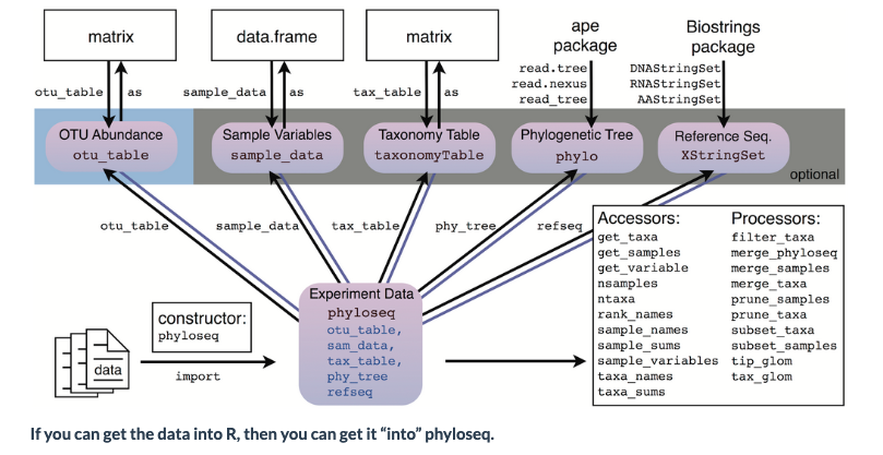
For examining the results of our analysis in R, we primarily be using the Phyloseq package, with some additional packages.
There are many possible file and data types that can be imported into Phyloseq:
To start off, we will load the R libraries we will need
# load the packages
library('phyloseq')
library('tibble')
library('ggplot2')
library('ape')
library('vegan')
We will do the work in the ‘plots’ directory, so in R, set that as the working directory
# set the working directory
setwd('../plots')
Now, we will put together all the elements to create a Phyloseq object
Import the frequency table
First we will import the frequency table.
import_table <- read.table('../otus/otu_frequency_table.tsv',header=TRUE,sep='\t',row.names=1, comment.char = "")
head(import_table)
| AM1 | AM2 | AM3 | AM4 | AM5 | AM6 | AS2 | AS3 | AS4 | AS5 | AS6 | |
|---|---|---|---|---|---|---|---|---|---|---|---|
| <int> | <int> | <int> | <int> | <int> | <int> | <int> | <int> | <int> | <int> | <int> | |
| OTU.1 | 723 | 3634 | 0 | 2907 | 171 | 1956 | 2730 | 2856 | 4192 | 3797 | 3392 |
| OTU.10 | 0 | 0 | 0 | 0 | 0 | 0 | 2223 | 0 | 0 | 1024 | 0 |
| OTU.11 | 1892 | 0 | 0 | 0 | 82 | 113 | 0 | 0 | 0 | 0 | 0 |
| OTU.12 | 0 | 1587 | 0 | 0 | 0 | 0 | 0 | 0 | 0 | 0 | 0 |
| OTU.13 | 0 | 0 | 0 | 0 | 0 | 0 | 0 | 0 | 0 | 1472 | 0 |
| OTU.14 | 0 | 0 | 0 | 0 | 0 | 0 | 0 | 0 | 0 | 0 | 1087 |
Now convert to a matrix for Phyloseq
otumat <- as.matrix(import_table)
head(otumat)
| AM1 | AM2 | AM3 | AM4 | AM5 | AM6 | AS2 | AS3 | AS4 | AS5 | AS6 | |
|---|---|---|---|---|---|---|---|---|---|---|---|
| OTU.1 | 723 | 3634 | 0 | 2907 | 171 | 1956 | 2730 | 2856 | 4192 | 3797 | 3392 |
| OTU.10 | 0 | 0 | 0 | 0 | 0 | 0 | 2223 | 0 | 0 | 1024 | 0 |
| OTU.11 | 1892 | 0 | 0 | 0 | 82 | 113 | 0 | 0 | 0 | 0 | 0 |
| OTU.12 | 0 | 1587 | 0 | 0 | 0 | 0 | 0 | 0 | 0 | 0 | 0 |
| OTU.13 | 0 | 0 | 0 | 0 | 0 | 0 | 0 | 0 | 0 | 1472 | 0 |
| OTU.14 | 0 | 0 | 0 | 0 | 0 | 0 | 0 | 0 | 0 | 0 | 1087 |
Now create an OTU object using the function otu_table
OTU <- otu_table(otumat, taxa_are_rows = TRUE)
head(OTU)
| AM1 | AM2 | AM3 | AM4 | AM5 | AM6 | AS2 | AS3 | AS4 | AS5 | AS6 | |
|---|---|---|---|---|---|---|---|---|---|---|---|
| OTU.1 | 723 | 3634 | 0 | 2907 | 171 | 1956 | 2730 | 2856 | 4192 | 3797 | 3392 |
| OTU.10 | 0 | 0 | 0 | 0 | 0 | 0 | 2223 | 0 | 0 | 1024 | 0 |
| OTU.11 | 1892 | 0 | 0 | 0 | 82 | 113 | 0 | 0 | 0 | 0 | 0 |
| OTU.12 | 0 | 1587 | 0 | 0 | 0 | 0 | 0 | 0 | 0 | 0 | 0 |
| OTU.13 | 0 | 0 | 0 | 0 | 0 | 0 | 0 | 0 | 0 | 1472 | 0 |
| OTU.14 | 0 | 0 | 0 | 0 | 0 | 0 | 0 | 0 | 0 | 0 | 1087 |
Import the taxonomy table
Now we will import the taxonomy table. This is the output from the Sintax analysis.
import_taxa <- read.table('../taxonomy/sintax_taxonomy.tsv',header=TRUE,sep='\t',row.names=1)
head(import_taxa)
| kingdom | phylum | class | order | family | genus | species | Confidence | |
|---|---|---|---|---|---|---|---|---|
| OTU.1 | Eukaryota | Chordata | Actinopteri | Scombriformes | Gempylidae | Thyrsites | Thyrsites_atun | 1.0000000 |
| OTU.2 | Eukaryota | Chordata | Actinopteri | Mugiliformes | Mugilidae | Aldrichetta | Aldrichetta_forsteri | 0.9999999 |
| OTU.3 | Eukaryota | Chordata | Actinopteri | Perciformes | Bovichtidae | Bovichtus | Bovichtus_variegatus | 0.9999979 |
| OTU.4 | Eukaryota | Chordata | Actinopteri | Blenniiformes | Tripterygiidae | Forsterygion | Forsterygion_lapillum | 1.0000000 |
| OTU.5 | Eukaryota | Chordata | Actinopteri | Labriformes | Labridae | Notolabrus | Notolabrus_fucicola | 0.9996494 |
| OTU.6 | Eukaryota | Chordata | Actinopteri | Blenniiformes | Tripterygiidae | Forsterygion | Forsterygion_lapillum | 1.0000000 |
Convert to a matrix:
taxonomy <- as.matrix(import_taxa)
Create a taxonomy class object
TAX <- tax_table(taxonomy)
Import the sample metadata
metadata <- read.table('../docs/sample_metadata.tsv',header = T,sep='\t',row.names = 1)
metadata
| fwd_barcode | rev_barcode | forward_primer | reverse_primer | location | temperature | salinity | sample | |
|---|---|---|---|---|---|---|---|---|
| <chr> | <chr> | <chr> | <chr> | <chr> | <int> | <int> | <chr> | |
| AM1 | GAAGAG | TAGCGTCG | GACCCTATGGAGCTTTAGAC | CGCTGTTATCCCTADRGTAACT | mudflats | 12 | 32 | AM1 |
| AM2 | GAAGAG | TCTACTCG | GACCCTATGGAGCTTTAGAC | CGCTGTTATCCCTADRGTAACT | mudflats | 14 | 32 | AM2 |
| AM3 | GAAGAG | ATGACTCG | GACCCTATGGAGCTTTAGAC | CGCTGTTATCCCTADRGTAACT | mudflats | 12 | 32 | AM3 |
| AM4 | GAAGAG | ATCTATCG | GACCCTATGGAGCTTTAGAC | CGCTGTTATCCCTADRGTAACT | mudflats | 10 | 32 | AM4 |
| AM5 | GAAGAG | ACAGATCG | GACCCTATGGAGCTTTAGAC | CGCTGTTATCCCTADRGTAACT | mudflats | 12 | 34 | AM5 |
| AM6 | GAAGAG | ATACTGCG | GACCCTATGGAGCTTTAGAC | CGCTGTTATCCCTADRGTAACT | mudflats | 10 | 34 | AM6 |
| AS2 | GAAGAG | AGATACTC | GACCCTATGGAGCTTTAGAC | CGCTGTTATCCCTADRGTAACT | shore | 12 | 32 | AS2 |
| AS3 | GAAGAG | ATGCGATG | GACCCTATGGAGCTTTAGAC | CGCTGTTATCCCTADRGTAACT | shore | 12 | 32 | AS3 |
| AS4 | GAAGAG | TGCTACTC | GACCCTATGGAGCTTTAGAC | CGCTGTTATCCCTADRGTAACT | shore | 10 | 34 | AS4 |
| AS5 | GAAGAG | ACGTCATG | GACCCTATGGAGCTTTAGAC | CGCTGTTATCCCTADRGTAACT | shore | 14 | 34 | AS5 |
| AS6 | GAAGAG | TCATGTCG | GACCCTATGGAGCTTTAGAC | CGCTGTTATCCCTADRGTAACT | shore | 10 | 34 | AS6 |
| ASN | GAAGAG | AGACGCTC | GACCCTATGGAGCTTTAGAC | CGCTGTTATCCCTADRGTAACT | negative | NA | NA | ASN |
As we are not using the negative control, we will remove it
metadata <- metadata[1:11,1:8]
tail(metadata)
| fwd_barcode | rev_barcode | forward_primer | reverse_primer | location | temperature | salinity | sample | |
|---|---|---|---|---|---|---|---|---|
| <chr> | <chr> | <chr> | <chr> | <chr> | <int> | <int> | <chr> | |
| AM6 | GAAGAG | ATACTGCG | GACCCTATGGAGCTTTAGAC | CGCTGTTATCCCTADRGTAACT | mudflats | 10 | 34 | AM6 |
| AS2 | GAAGAG | AGATACTC | GACCCTATGGAGCTTTAGAC | CGCTGTTATCCCTADRGTAACT | shore | 12 | 32 | AS2 |
| AS3 | GAAGAG | ATGCGATG | GACCCTATGGAGCTTTAGAC | CGCTGTTATCCCTADRGTAACT | shore | 12 | 32 | AS3 |
| AS4 | GAAGAG | TGCTACTC | GACCCTATGGAGCTTTAGAC | CGCTGTTATCCCTADRGTAACT | shore | 10 | 34 | AS4 |
| AS5 | GAAGAG | ACGTCATG | GACCCTATGGAGCTTTAGAC | CGCTGTTATCCCTADRGTAACT | shore | 14 | 34 | AS5 |
| AS6 | GAAGAG | TCATGTCG | GACCCTATGGAGCTTTAGAC | CGCTGTTATCCCTADRGTAACT | shore | 10 | 34 | AS6 |
Create a Phyloseq sample_data-class
META <- sample_data(metadata)
Create a Phyloseq object
Now that we have all the components, it is time to create a Phyloseq object
physeq <- phyloseq(OTU,TAX,META)
physeq
    phyloseq-class experiment-level object
    otu_table()   OTU Table:         [ 33 taxa and 11 samples ]
    sample_data() Sample Data:       [ 11 samples by 8 sample variables ]
    tax_table()   Taxonomy Table:    [ 33 taxa by 8 taxonomic ranks ]
One last thing we will do is to convert two of the metadata variables from continuous to ordinal. This will help us graph these fields later
sample_data(physeq)$temperature <- as(sample_data(physeq)$temperature, "character")

sample_data(physeq)$salinity <- as(sample_data(physeq)$salinity, "character")
Initial data inspection
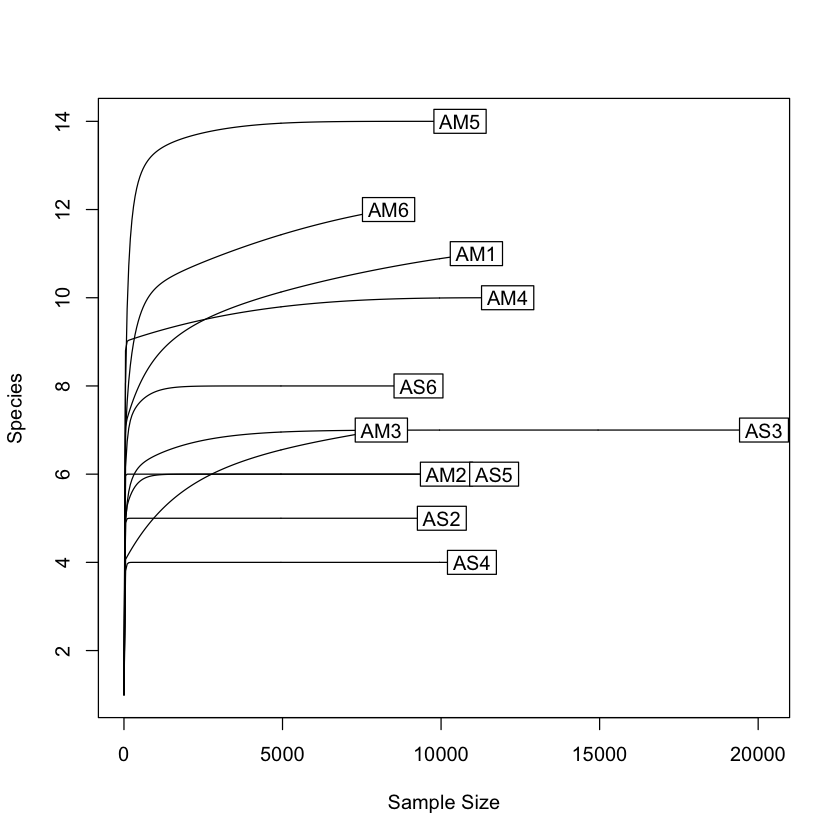
Now that we have our Phyloseq object, we will take a look at it. One of the first steps is to check alpha rarefaction of species richness. This is done to show that there has been sufficient sequencing to detect most species (OTUs).
rarecurve(t(otu_table(physeq)), step=50, cex=1)
create a bar plot of abundance
plot_bar(physeq)
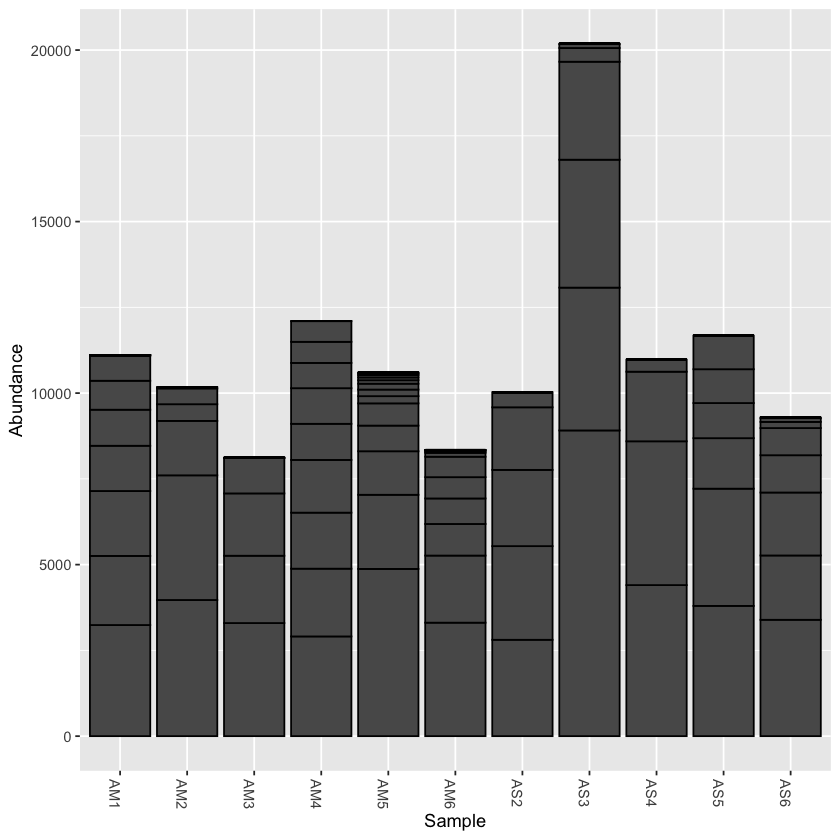
print(min(sample_sums(physeq)))
print(max(sample_sums(physeq)))
    [1] 8117
    [1] 20184
Rarefy the data
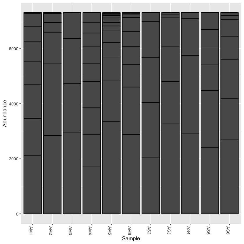
From the initial look at the data, it is obvious that the sample AS3 has about twice as many reads as any of the other samples. We can use rarefaction to simulate an even number of reads per sample. Rarefying the data is preferred for some analyses, though there is some debate. We will create a rarefied version of the Phyloseq object.
we will rarefy the data around 90% of the lowest sample
physeq.rarefied <- rarefy_even_depth(physeq, rngseed=1, sample.size=0.9*min(sample_sums(physeq)), replace=F)
    `set.seed(1)` was used to initialize repeatable random subsampling.

    Please record this for your records so others can reproduce.

    Try `set.seed(1); .Random.seed` for the full vector

    ...
now plot the rarefied version
plot_bar(physeq.rarefied)
Saving your work to files
You can save the Phyloseq object you just created, and then import it into another R session later. This way you do not have to re-import all the components separately.
Also, below are a couple of examples of saving graphs. There are many options for this that you can explore to create publication-quality graphics of your results
Save the phyloseq object
saveRDS(physeq, 'fish_phyloseq.rds')
Also save the rarefied version
saveRDS(physeq.rarefied, 'fish_phyloseq_rarefied.rds')
To later read the Phyloseq object into your R session:
first the original
physeq <- readRDS('fish_phyloseq.rds')
print(physeq)
Saving a graph to file
# open a pdf file
pdf('species_richness_plot.pdf')
# run the plot, or add the saved one
rarecurve(t(otu_table(physeq)), step=50, cex=1.5, col='blue',lty=2)
# close the pdf
dev.off()
pdf: 2
there are other graphic formats that you can use
jpeg("species_richness_plot.jpg", width = 800, height = 800)
rarecurve(t(otu_table(physeq)), step=50, cex=1.5, col='blue',lty=2)
dev.off()
pdf: 2
Key Points
Phyloseq has many functions to explore metabarcoding data
Results from early lessons must be converted to a matrix
Phyloseq is integrated with ggplot to expand graphic output