Statistics and Graphing with R
Overview
Teaching: 10 min
Exercises: 50 minQuestions
How do I use ggplot and other programs with Phyloseq?
What statistical approaches do I use to explore my metabarcoding results?
Objectives
Create bar plots of taxonomy and use them to show differences across the metadata
Create distance ordinations and use them to make PCoA plots
Make subsets of the data to explore specific aspects of your results
In this lesson there are several examples for plotting the results of your analysis. As mentioned in the previous lesson, here are some links with additional graphing examples:
-
The Phyloseq web page has many good tutorials
-
The Micca pipeline has a good intro tutorial for Phyloseq
-
Remember, if you are starting a new notebook, to set the working directory and read in the Phyloseq object:
setwd(../plots)
# load the packages
library('phyloseq')
library('tibble')
library('ggplot2')
library('ape')
library('vegan')

physeq <- readRDS('fish_phyloseq.rds')
print(physeq)
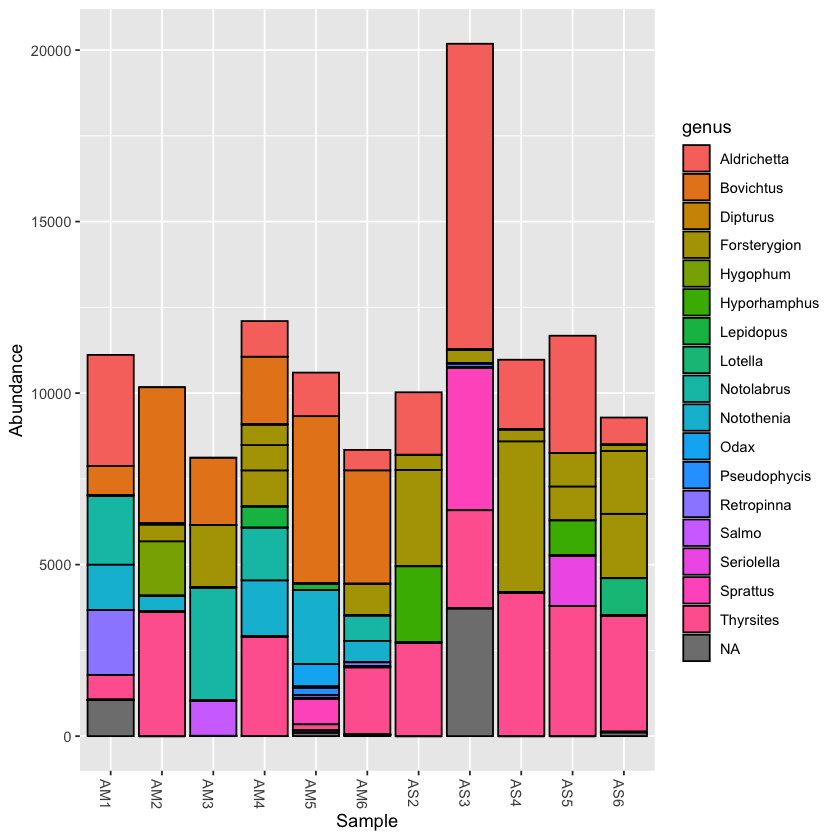
Plotting taxonomy
Using the plot_bar function, we can plot the relative abundance of taxa across samples
plot_bar(physeq, fill='genus')
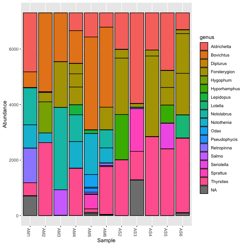
Plotting the taxonomy with the rarefied dataset can help to compare abundance across samples
plot_bar(physeq.rarefied, fill='genus')
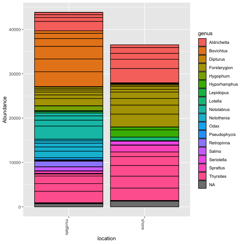
You can collapse the frequency counts across metadata categories, such as location
plot_bar(physeq.rarefied, x='location', fill='genus')
Exercise: collapse counts around temperature
Try to collapse counts around another metadata category, like temperature. Then try filling at a different taxonomic level, like order or family
Solution
plot_bar(physeq.rarefied, x='temperature', fill='family')
Incorporate ggplot into your Phyloseq graph
Now we will try to add ggplot elements to the graph
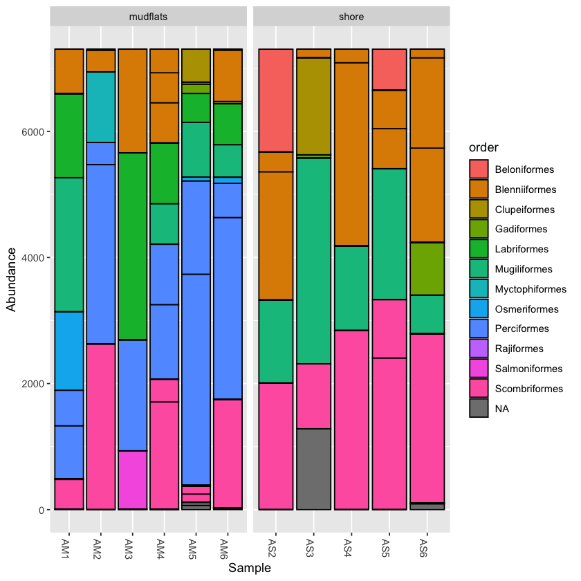
Add ggplot facet_wrap tool to graph
Try using facet_wrap to break your plot into separate parts
Hint: First save your plot to a variable, then you can add to it
Solution
barplot1 <- plot_bar(physeq.rarefied, fill='order')

barplot1 + facet_wrap(~location, scales="free_x",nrow=1)
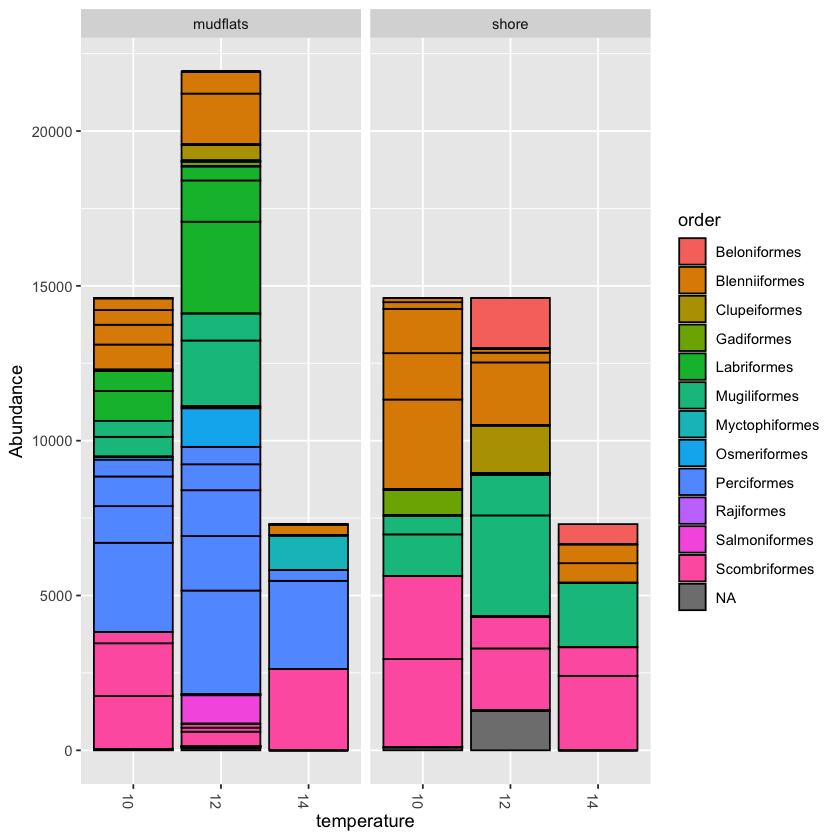
Combine visuals to present more information
Now that you can use facet_wrap, try to show both location and temperature in a single graph.
Hint: Try to combine from the above two techniques
Solution
barplot2 <- plot_bar(physeq.rarefied, x="temperature", fill='order') +
facet_wrap(~location, scales="free_x", nrow=1)

barplot2
Community ecology
The Phyloseq package has many functions for exploring diversity within and between samples. This includes multiple methods of calculating distance matrices between samples.
An ongoing debate with metabarcoding data is whether relative frequency of OTUs should be taken into account, or whether they should be scored as presence or absence. Phyloseq allows you to calculate distance using both qualitative (i.e. presence/absence) and quantitative (abundance included) measures, taken from community ecology diversity statistics.
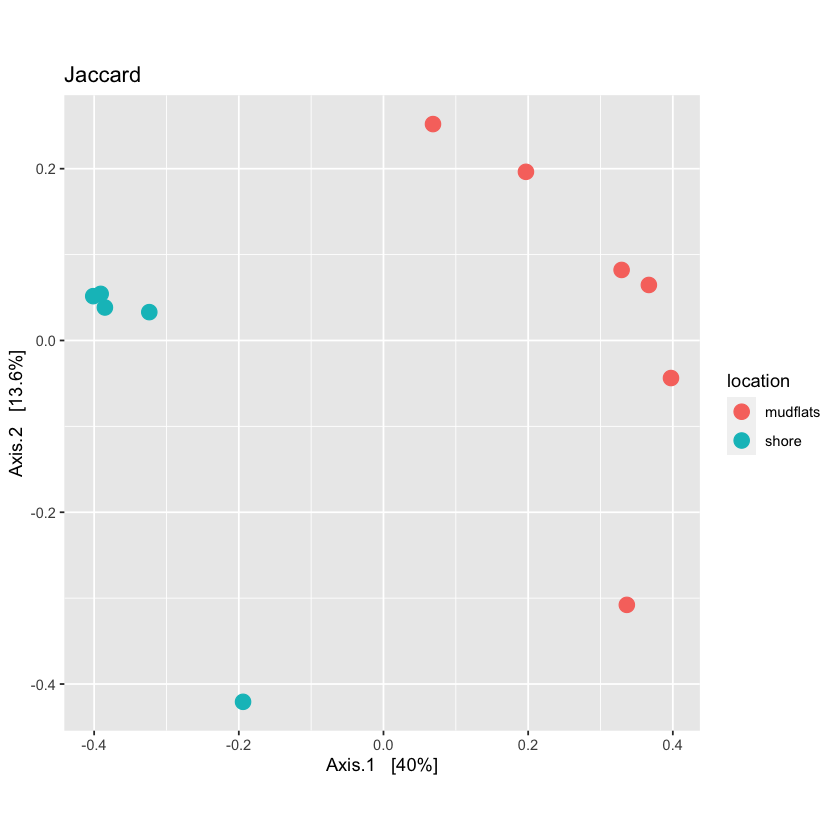
For qualitative distance use the Jaccard method
jac_dist <- distance(physeq.rarefied, method = "jaccard", binary = TRUE)
jac_dist
jac_dist
              AM1       AM2       AM3       AM4       AM5       AM6       AS2
    AM2 0.7692308
    AM3 0.6923077 0.8181818
    AM4 0.5714286 0.6666667 0.7857143
    AM5 0.6666667 0.8235294 0.7647059 0.6666667
    AM6 0.4285714 0.8000000 0.7333333 0.6250000 0.5555556
    AS2 0.8461538 0.7777778 0.9090909 0.7500000 0.8823529 0.8666667
    AS3 0.8666667 0.8181818 0.9230769 0.8666667 0.7647059 0.8823529 0.6666667
    AS4 0.8333333 0.7500000 0.9000000 0.7272727 0.8750000 0.8571429 0.2000000
    AS5 0.8571429 0.8000000 0.9166667 0.7692308 0.8888889 0.8750000 0.1666667
    AS6 0.8750000 0.8333333 0.9285714 0.8000000 0.9000000 0.8888889 0.5555556
              AS3       AS4       AS5
    AM2
    AM3
    AM4
    AM5
    AM6
    AS2
    AS3
    AS4 0.6250000
    AS5 0.7000000 0.3333333
    AS6 0.7500000 0.5000000 0.6000000
Now you can run the ordination function in Phyloseq and then plot it.
qual_ord <- ordinate(physeq.rarefied, method="PCoA", distance=jac_dist)
plot_jac <- plot_ordination(physeq.rarefied, qual_ord, color="location", title='Jaccard') + theme(aspect.ratio=1) + geom_point(size=4)
plot_jac
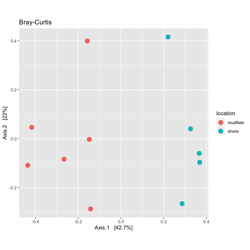
Using quantitative distances
For quantitative distance use the Bray-Curtis method:
bc_dist <- distance(physeq.rarefied, method = "bray", binary = FALSE)
Now run ordination on the quantitative distances and plot them
Also try to make the points of the graph smaller
Solution
quant_ord <- ordinate(physeq.rarefied, method="PCoA", distance=bc_dist)plot_bc <- plot_ordination(physeq.rarefied, quant_ord, color="location", title='Bray-Curtis') + theme(aspect.ratio=1) + geom_point(size=3) plot_bc
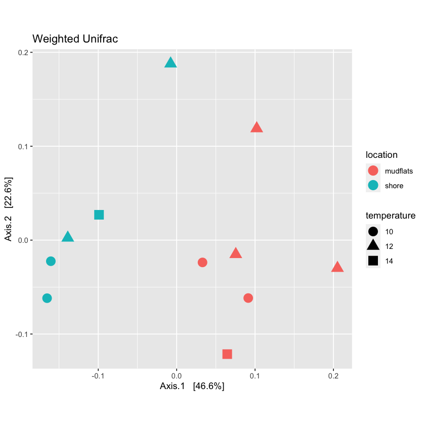
View multiple variables on a PCoA plot
Phyloseq allows you to graph multiple characteristics. Try to plot location by color and temperature by shape
Solution
plot_locTemp <- plot_ordination(physeq.rarefied, quant_ord, color="location", shape='temperature', title="Jaccard Location and Temperature") +
theme(aspect.ratio=1) +
geom_point(size=4)

plot_locTemp
Permutational ANOVA
Phyloseq includes the adonis function to run a PERMANOVA to determine if OTUs from specific metadata fields are significantly different from each other.
adonis(bc_dist ~ sample_data(physeq.rarefied)$location)
    Call:
    adonis(formula = bc_dist ~ sample_data(physeq.rarefied)$location)

    Permutation: free
    Number of permutations: 999

    Terms added sequentially (first to last)

                                          Df SumsOfSqs  MeanSqs F.Model      R2
    sample_data(physeq.rarefied)$location  1   0.13144 0.131438   5.938 0.39751
    Residuals                              9   0.19921 0.022135         0.60249
    Total                                 10   0.33065                  1.00000
                                          Pr(>F)
    sample_data(physeq.rarefied)$location  0.002 **
    Residuals
    Total
    ---
    Signif. codes:  0 ‘***’ 0.001 ‘**’ 0.01 ‘*’ 0.05 ‘.’ 0.1 ‘ ’ 1
Is temperature significantly different?
Run PERMANOVA on the temperature variable
Solution
adonis(bc_dist ~ sample_data(physeq.rarefied)$temperature)Call: adonis(formula = bc_dist ~ sample_data(physeq.rarefied)$temperature) Permutation: free Number of permutations: 999 Terms added sequentially (first to last) Df SumsOfSqs MeanSqs F.Model R2 sample_data(physeq.rarefied)$temperature 2 0.06606 0.033031 0.99869 0.19979 Residuals 8 0.26459 0.033074 0.80021 Total 10 0.33065 1.00000 Pr(>F) sample_data(physeq.rarefied)$temperature 0.441 Residuals TotalTemperature is not significantly different across samples
Subsetting data
It is possible to take subsets of the Phyloseq object you have created. You can subset by taxa or samples.
Subsetting by taxonomy
Often there are so many taxonomic groups represented, that it is useful to create a subset of the data that contains only OTUs belonging to a taxonomic rank. This is done with the subset_taxa function. In the example dataset provided, there are not too many taxa included, but for larger datasets this can be very useful
scomb <- subset_taxa(physeq, order=='Scombriformes')
the subsetted database is still a valid Phyloseq object:
scomb
    phyloseq-class experiment-level object
    otu_table()   OTU Table:         [ 3 taxa and 11 samples ]
    sample_data() Sample Data:       [ 11 samples by 8 sample variables ]
    tax_table()   Taxonomy Table:    [ 3 taxa by 8 taxonomic ranks ]
plot_bar(scomb, fill='species')
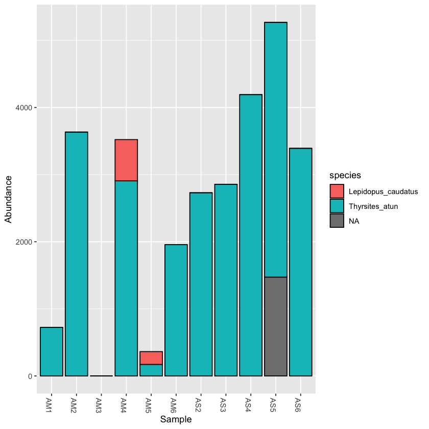
Exercise: take a subset of a taxon and plot it
Subset samples
Now we will try to make a subset of the Phyloseq object based on a field from the sample metadata table.
First, let’s look at the metadata:
sample_data(physeq)
| fwd_barcode | rev_barcode | forward_primer | reverse_primer | location | temperature | salinity | sample | |
|---|---|---|---|---|---|---|---|---|
| <chr> | <chr> | <chr> | <chr> | <chr> | <fct> | <fct> | <chr> | |
| AM1 | GAAGAG | TAGCGTCG | GACCCTATGGAGCTTTAGAC | CGCTGTTATCCCTADRGTAACT | mudflats | 12 | 32 | AM1 |
| AM2 | GAAGAG | TCTACTCG | GACCCTATGGAGCTTTAGAC | CGCTGTTATCCCTADRGTAACT | mudflats | 14 | 32 | AM2 |
| AM3 | GAAGAG | ATGACTCG | GACCCTATGGAGCTTTAGAC | CGCTGTTATCCCTADRGTAACT | mudflats | 12 | 32 | AM3 |
| AM4 | GAAGAG | ATCTATCG | GACCCTATGGAGCTTTAGAC | CGCTGTTATCCCTADRGTAACT | mudflats | 10 | 32 | AM4 |
| AM5 | GAAGAG | ACAGATCG | GACCCTATGGAGCTTTAGAC | CGCTGTTATCCCTADRGTAACT | mudflats | 12 | 34 | AM5 |
| AM6 | GAAGAG | ATACTGCG | GACCCTATGGAGCTTTAGAC | CGCTGTTATCCCTADRGTAACT | mudflats | 10 | 34 | AM6 |
| AS2 | GAAGAG | AGATACTC | GACCCTATGGAGCTTTAGAC | CGCTGTTATCCCTADRGTAACT | shore | 12 | 32 | AS2 |
| AS3 | GAAGAG | ATGCGATG | GACCCTATGGAGCTTTAGAC | CGCTGTTATCCCTADRGTAACT | shore | 12 | 32 | AS3 |
| AS4 | GAAGAG | TGCTACTC | GACCCTATGGAGCTTTAGAC | CGCTGTTATCCCTADRGTAACT | shore | 10 | 34 | AS4 |
| AS5 | GAAGAG | ACGTCATG | GACCCTATGGAGCTTTAGAC | CGCTGTTATCCCTADRGTAACT | shore | 14 | 34 | AS5 |
| AS6 | GAAGAG | TCATGTCG | GACCCTATGGAGCTTTAGAC | CGCTGTTATCCCTADRGTAACT | shore | 10 | 34 | AS6 |
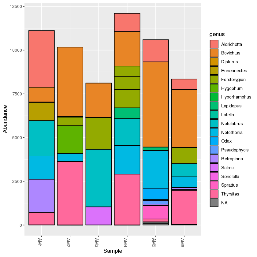
The command is similar to the subset_taxa command. For example, if we want to only analyse the samples found in the mudflats:
mud <- subset_samples(physeq, location=='mudflats')

mud
The output is still a Phyloseq object:
    phyloseq-class experiment-level object
    otu_table()   OTU Table:         [ 33 taxa and 6 samples ]
    sample_data() Sample Data:       [ 6 samples by 8 sample variables ]
    tax_table()   Taxonomy Table:    [ 33 taxa by 8 taxonomic ranks ]
A taxonomy bar plot will only show the mudflats samples:
plot_bar(mud, fill='genus')
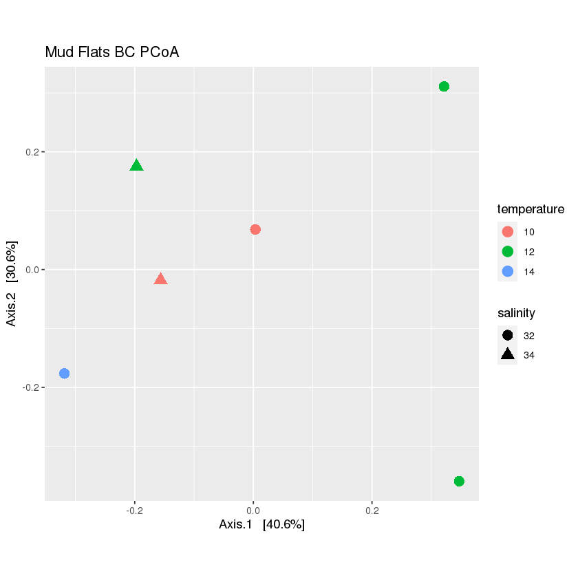
Exercise: create a PCoA plot of the mudflats subset
Hint: is there anything that should be done with the data before plotting?
Solution
First, rarefy the new dataset:
mud.rarefied <- rarefy_even_depth(mud, rngseed=1, sample.size=0.9*min(sample_sums(mud)), replace=F)Now, calculate the distance and ordination
mud_dist <- distance(mud.rarefied, method = 'bray', binary=FALSE)

mud_ord <- ordinate(mud.rarefied, method="PCoA", distance=mud_dist)
Finally, plot the ordination
plot_mud <- plot_ordination(mud.rarefied, mud_ord, color='temperature',shape='salinity', title="Mud Flats BC PCoA")+
theme(aspect.ratio=1)+ geom_point(size=4)

plot_mud
Merge OTUs by taxa
The final function we will present is to merge the OTUs by taxonomy. You will notice that there are often multiple OTUs that are assigned to a single species or genus. This can be due to multiple factors, such as sequence error, gaps in the reference database, or a species that varies in the target region. If you are interested in focusing on the taxonomy, then it is useful to merge OTUs that assign to the same taxon. Fortunately, Phyloseq provides a useful function to do this.
We will merge all OTUs at the lowest taxonomic level
phyMerge <- tax_glom(physeq, taxrank = 'species',NArm = T)
Now have a look at the taxonomy table. You should see that there are fewer OTUs.
tax_table(phyMerge)
| kingdom | phylum | class | order | family | genus | species | Confidence | |
|---|---|---|---|---|---|---|---|---|
| OTU.8 | Eukaryota | Chordata | Actinopteri | Clupeiformes | Clupeidae | Sprattus | Sprattus_muelleri | NA |
| OTU.21 | Eukaryota | Chordata | Actinopteri | Clupeiformes | Clupeidae | Sprattus | Sprattus_antipodum | NA |
| OTU.17 | Eukaryota | Chordata | Actinopteri | Blenniiformes | Tripterygiidae | Enneanectes | Enneanectes_carminalis | NA |
| OTU.4 | Eukaryota | Chordata | Actinopteri | Blenniiformes | Tripterygiidae | Forsterygion | Forsterygion_lapillum | NA |
| OTU.11 | Eukaryota | Chordata | Actinopteri | Osmeriformes | Retropinnidae | Retropinna | Retropinna_retropinna | NA |
| OTU.10 | Eukaryota | Chordata | Actinopteri | Beloniformes | Hemiramphidae | Hyporhamphus | Hyporhamphus_melanochir | NA |
| OTU.3 | Eukaryota | Chordata | Actinopteri | Perciformes | Bovichtidae | Bovichtus | Bovichtus_variegatus | NA |
| OTU.7 | Eukaryota | Chordata | Actinopteri | Perciformes | Nototheniidae | Notothenia | Notothenia_angustata | NA |
| OTU.2 | Eukaryota | Chordata | Actinopteri | Mugiliformes | Mugilidae | Aldrichetta | Aldrichetta_forsteri | NA |
| OTU.5 | Eukaryota | Chordata | Actinopteri | Labriformes | Labridae | Notolabrus | Notolabrus_fucicola | NA |
| OTU.22 | Eukaryota | Chordata | Actinopteri | Labriformes | Odacidae | Odax | Odax_pullus | NA |
| OTU.14 | Eukaryota | Chordata | Actinopteri | Gadiformes | Moridae | Lotella | Lotella_rhacina | NA |
| OTU.23 | Eukaryota | Chordata | Actinopteri | Gadiformes | Moridae | Pseudophycis | Pseudophycis_barbata | NA |
| OTU.19 | Eukaryota | Chordata | Actinopteri | Scombriformes | Trichiuridae | Lepidopus | Lepidopus_caudatus | NA |
| OTU.1 | Eukaryota | Chordata | Actinopteri | Scombriformes | Gempylidae | Thyrsites | Thyrsites_atun | NA |
| OTU.12 | Eukaryota | Chordata | Actinopteri | Myctophiformes | Myctophidae | Hygophum | Hygophum_hanseni | NA |
Exercise
In the previous example, you might have noticed that any OTU that was not resolved to species (i.e. ‘NA’ in the species column) was removed from the table. Try to rerun the function, keeping all the unresolved species.
Solution
phyMergeNA <- tax_glom(physeq, taxrank = 'species',NArm = F)tax_table(phyMergeNA)
A taxonomyTable: 23 × 8 of type chr kingdom phylum class order family genus species Confidence OTU.33 Eukaryota Chordata NA NA NA NA NA NA OTU.8 Eukaryota Chordata Actinopteri Clupeiformes Clupeidae Sprattus Sprattus_muelleri NA OTU.21 Eukaryota Chordata Actinopteri Clupeiformes Clupeidae Sprattus Sprattus_antipodum NA OTU.29 Eukaryota Chordata Actinopteri Clupeiformes Clupeidae Sprattus NA NA OTU.17 Eukaryota Chordata Actinopteri Blenniiformes Tripterygiidae Enneanectes Enneanectes_carminalis NA OTU.4 Eukaryota Chordata Actinopteri Blenniiformes Tripterygiidae Forsterygion Forsterygion_lapillum NA OTU.11 Eukaryota Chordata Actinopteri Osmeriformes Retropinnidae Retropinna Retropinna_retropinna NA OTU.15 Eukaryota Chordata Actinopteri Salmoniformes Salmonidae Salmo NA NA OTU.10 Eukaryota Chordata Actinopteri Beloniformes Hemiramphidae Hyporhamphus Hyporhamphus_melanochir NA OTU.3 Eukaryota Chordata Actinopteri Perciformes Bovichtidae Bovichtus Bovichtus_variegatus NA OTU.7 Eukaryota Chordata Actinopteri Perciformes Nototheniidae Notothenia Notothenia_angustata NA OTU.2 Eukaryota Chordata Actinopteri Mugiliformes Mugilidae Aldrichetta Aldrichetta_forsteri NA OTU.9 Eukaryota Chordata Actinopteri NA NA NA NA NA OTU.5 Eukaryota Chordata Actinopteri Labriformes Labridae Notolabrus Notolabrus_fucicola NA OTU.22 Eukaryota Chordata Actinopteri Labriformes Odacidae Odax Odax_pullus NA OTU.31 Eukaryota Chordata Chondrichthyes Rajiformes Rajidae Dipturus NA NA OTU.14 Eukaryota Chordata Actinopteri Gadiformes Moridae Lotella Lotella_rhacina NA OTU.23 Eukaryota Chordata Actinopteri Gadiformes Moridae Pseudophycis Pseudophycis_barbata NA OTU.28 Eukaryota Chordata Actinopteri Gadiformes Moridae Pseudophycis NA NA OTU.19 Eukaryota Chordata Actinopteri Scombriformes Trichiuridae Lepidopus Lepidopus_caudatus NA OTU.1 Eukaryota Chordata Actinopteri Scombriformes Gempylidae Thyrsites Thyrsites_atun NA OTU.13 Eukaryota Chordata Actinopteri Scombriformes Centrolophidae Seriolella NA NA OTU.12 Eukaryota Chordata Actinopteri Myctophiformes Myctophidae Hygophum Hygophum_hanseni NA
Exercise
What would happen if you set the
taxrankparameter in thetax_glomfunction to a higher taxonomic level, like family?Solution
phyMergeFAM <- tax_glom(physeq, taxrank = 'family',NArm = T)

tax_table(phyMergeFAM)
A taxonomyTable: 16 × 8 of type chr kingdom phylum class order family genus species Confidence OTU.8 Eukaryota Chordata Actinopteri Clupeiformes Clupeidae NA NA NA OTU.4 Eukaryota Chordata Actinopteri Blenniiformes Tripterygiidae NA NA NA OTU.11 Eukaryota Chordata Actinopteri Osmeriformes Retropinnidae NA NA NA OTU.15 Eukaryota Chordata Actinopteri Salmoniformes Salmonidae NA NA NA OTU.10 Eukaryota Chordata Actinopteri Beloniformes Hemiramphidae NA NA NA OTU.3 Eukaryota Chordata Actinopteri Perciformes Bovichtidae NA NA NA OTU.7 Eukaryota Chordata Actinopteri Perciformes Nototheniidae NA NA NA OTU.2 Eukaryota Chordata Actinopteri Mugiliformes Mugilidae NA NA NA OTU.5 Eukaryota Chordata Actinopteri Labriformes Labridae NA NA NA OTU.22 Eukaryota Chordata Actinopteri Labriformes Odacidae NA NA NA OTU.31 Eukaryota Chordata Chondrichthyes Rajiformes Rajidae NA NA NA OTU.14 Eukaryota Chordata Actinopteri Gadiformes Moridae NA NA NA OTU.19 Eukaryota Chordata Actinopteri Scombriformes Trichiuridae NA NA NA OTU.1 Eukaryota Chordata Actinopteri Scombriformes Gempylidae NA NA NA OTU.13 Eukaryota Chordata Actinopteri Scombriformes Centrolophidae NA NA NA OTU.12 Eukaryota Chordata Actinopteri Myctophiformes Myctophidae NA NA NA
Key Points
The Phyloseq package has many useful features to conduct statistical analyses of your data