Introduction to NeSI
Overview
Teaching: 15 min
Exercises: 15 minQuestions
How can I log onto Jupyter hub notebooks hosted on NeSI
Objectives
Understand how to log into Jupyter hub on NeSI
Introduction to NeSI
WARNING- We do not recommend using Internet Explorer to accss NeSI JupyterHub
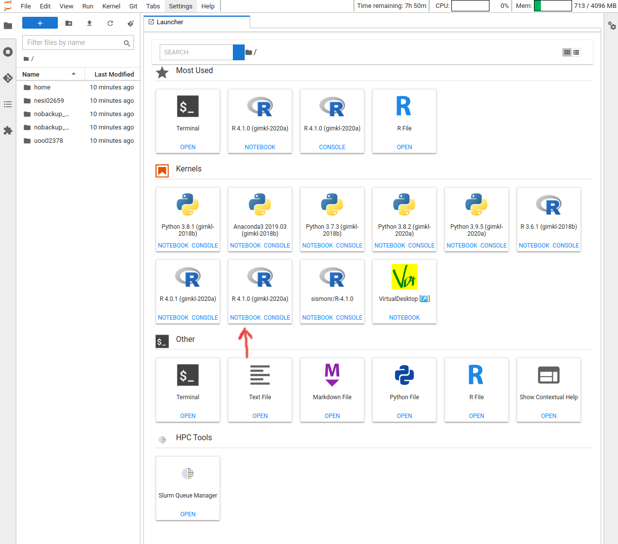
- Follow https://jupyter.nesi.org.nz/hub/login
- Enter NeSI username, HPC password and 6 digit second factor token
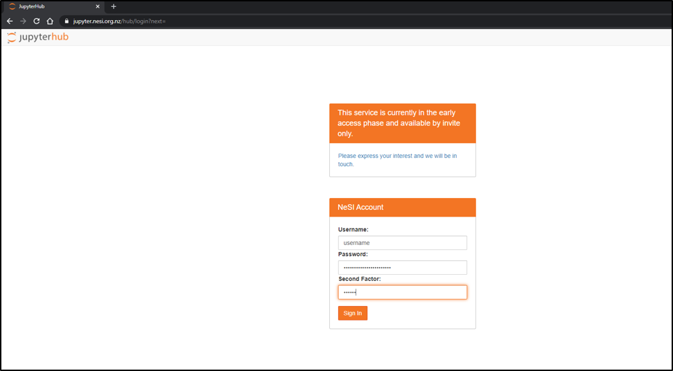
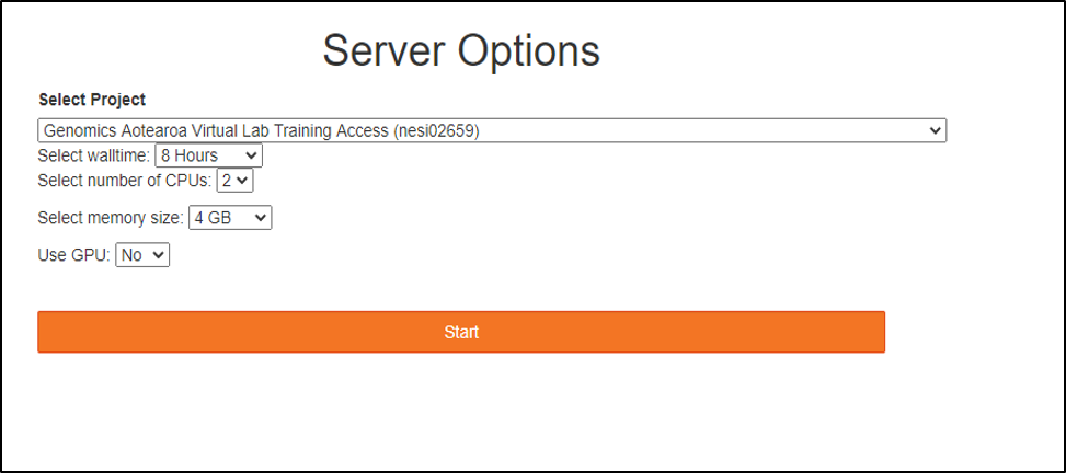
- Choose server options as below OR as required for the session
Project code should be nesi02659 (select from drop down list), Number of CPUs and memory size will remain unchanged. However, select the approriate Wall time based on the projected length of a session
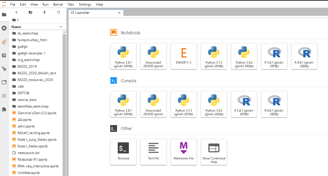
- Jupyter Launcher screen
Getting data onto/off of NeSI
For small files (a few megabytes) you can use the upload button on Jupyter hub in the file explorer pane. For downloading (small files) use the navigation pane to find the file you would like, right click and then select to download.
Both upload and download through Jupyter Hub is done through the browser and not recommended for larger files ( >100 MB)
For moving larger data onto or off of NeSI the use of globus is recommended.
Key Points
NeSI provides interactive access through Jupyter hub
Introduction to the UNIX shell
Overview
Teaching: 90 min
Exercises: 25 minQuestions
What is a command shell and why would I use one?
How can I see what files and directories I have?
How can I use loops and scripts to my advantage?
Objectives
Use the shell to navigate directories
Perform operations on files in directories outside your working directory
Interconvert between relative and absolute paths
View, search within, copy, move, and rename files. Create new directories.
Construct command pipelines with two or more stages.
Use for loops to run the same command for several input files.
Introduction to Unix commandline (BASH)
Learning objectives:
These introductory notes are adapted from The Carpentries Introduction to the Command Line for Genomics lessons
Introducing the Shell
A shell is a computer program that presents a command line interface which allows you to control your computer using commands entered with a keyboard instead of controlling graphical user interfaces (GUIs) with a mouse/keyboard combination.
Many bioinformatics tools can only be used through a command line interface, or have extra capabilities in the command line version that are not available in the GUI. This is true, for example, of BLAST, which offers many advanced functions only accessible to users who know how to use a shell.
- The shell makes your work less boring. In bioinformatics you often need to do the same set of tasks with a large number of files. Learning the shell will allow you to automate those repetitive tasks and leave you free to do more exciting things.
- The shell makes your work less error-prone. When humans do the same thing a hundred different times (or even ten times), they’re likely to make a mistake. Your computer can do the same thing a thousand times with no mistakes.
- The shell makes your work more reproducible. When you carry out your work in the command-line (rather than a GUI), your computer keeps a record of every step that you’ve carried out, which you can use to re-do your work when you need to. It also gives you a way to communicate unambiguously what you’ve done, so that others can check your work or apply your process to new data.
- Many bioinformatic tasks require large amounts of computing power and can’t realistically be run on your own machine. These tasks are best performed using remote computers or cloud computing, which can only be accessed through a shell.
In this lesson you will learn how to use the command line interface to move around in your file system.
Open up a terminal in Juypter.
[matt.bixley@wbg004 ~/.jupyter/jobs/22861436] $
Note you will automatically start off in a directory related to the slurm job running your Jupyter session e.g.
~/.jupyter/jobs/22861436
The dollar sign is a prompt, which shows us that the shell is waiting for input; your shell may use a different character as a prompt and may add information before the prompt. When typing commands, either from these lessons or from other sources, do not type the prompt, only the commands that follow it.
Let’s find out where we are by running a command called pwd
(which stands for “print working directory”).
At any moment, our current working directory
is our current default directory,
i.e.,
the directory that the computer assumes we want to run commands in,
unless we explicitly specify something else.
Here, the computer’s response is /home/yourname/.jupyter/jobs/yourjobid,
name and the number you see will be different and relates to your username and the
specific Jupyter session running on NeSI.
$ pwd
/home/matt.bixley/.jupyter/jobs/22861436
Let’s look at how our file system is organized. We can see what files and subdirectories are in this directory by running ls,
which stands for “listing”:
$ ls
home nesi02659 nobackup_nesi02659
ls prints the names of the files and directories in the current directory in
alphabetical order,
arranged neatly into columns.
We can also add flags to our commands which will modify the behaviour of the command.
$ ls -l
total 3
lrwxrwxrwx 1 matt.bixley matt.bixley 19 Oct 18 21:02 home -> /home/matt.bixley
lrwxrwxrwx 1 matt.bixley matt.bixley 23 Oct 18 21:02 nesi02659 -> /nesi/project/nesi02659
lrwxrwxrwx 1 matt.bixley matt.bixley 24 Oct 18 21:02 nobackup_nesi02659 -> /nesi/nobackup/nesi02659
The -> in this output tells us that we have some shortcut links in this directory.
homein this case is a short cut to our actualhomedirectorynesi02659is a shortcut to our project on the nesi filesystem.nobackup_nesi002659is a shortcut to project directory that isn’t backed up
Full vs. Relative Paths
Directories can be specified using either a relative path or a full absolute path. The directories on the computer are arranged into a hierarchy. The full path tells you where a directory is in that hierarchy.
- A full path will always start with
/- also known as the root - A relative path is the path based on what you can see in your current directory
Here is an example of how the workshop directory hierarchy is set up:
/
|-- home/
  |-- matt.bixley/
    |-- obss_2021/
      |-- enda/
      |-- gbs/
      |-- genomic_dna/
      |-- intro_bash/
      |-- intro_r/
      `-- rnaseq/
Home
Your home directory is where your user account lives on the filesystem and is found at /home/yourname. Because your home directory special to you, it can also be referred to using ~/ which bash will automatically convert to the full path of /home/yourname.
Navigating Files and Directories
The command to change locations in our file system is cd, followed by a
directory name to change our working directory.
cd stands for “change directory”.
Lets use cd to navigate to our home directory using ~/ to represent our home.
$ cd ~/
$ pwd
/home/matt.bixley
Using
cdwithout specifying a directory will by default send you to your home directory
This is the full name of your home directory. This tells you that you
are in a directory called matt.bixley, which sits inside a directory called
home which sits inside the very top directory in the hierarchy. The
very top of the hierarchy is a directory called / which is usually
referred to as the root directory. So, to summarize: matt.bixley is a
directory in home which is a directory in / (root).
Let’s look at what is in your home directory:
ls
obss_2021
obss_2021 is where we will be working out of for the entirity of the workshop. Lets change into that directory now using a relative path.
cd obss_2021
We can make the ls output from above, more comprehensible by using the flag -F,
which tells ls to add a trailing / to the names of directories:
$ ls -F
edna/ gbs/ genomic_dna/ intro_bash/ intro_r/ rnaseq/
Anything with a “/” after it is a directory. Things with a “*” after them are programs. If there are no decorations, it’s a file.
/home/matt.bixley/obss_2021
We have a special command to tell the computer to move us back or up one directory level.
$ cd ..
$ pwd
You will see:
/home/yourname
Now enter the following command:
$ cd /home/yourname/obss_2021/intro_bash/shell_data/
This jumps forward multiple levels to the shell_data directory.
Now go back to the home directory with cd or cd ~
$ cd
You can also navigate to the shell_data directory using:
$ cd obss_2021/intro_bash/shell_data
These two commands have the same effect, they both take us to the shell_data directory.
The first uses the absolute path, giving the full address from the home directory. The
second uses a relative path, giving only the address from the working directory. A full
path always starts with a /. A relative path does not.
A relative path is like getting directions from someone on the street. They tell you to “go right at the stop sign, and then turn left on Main Street”. That works great if you’re standing there together, but not so well if you’re trying to tell someone how to get there from another country. A full path is like GPS coordinates. It tells you exactly where something is no matter where you are right now.
Examining Files
We now know how to switch directories, run programs, and look at the contents of directories, but how do we look at the contents of files?
One way to examine a file is to print out all of the
contents using the program cat.
Enter the following command from within the untrimmed_fastq directory:
$ cat SRR098026.fastq
This will print out all of the contents of the SRR098026.fastq to the screen.
Enter the following command:
$ less SRR097977.fastq
Some navigation commands in less:
| key | action |
|---|---|
| Space | to go forward |
| b | to go backward |
| g | to go to the beginning |
| G | to go to the end |
| q | to quit |
less also gives you a way of searching through files. Use the
“/” key to begin a search. Enter the word you would like
to search for and press enter. The screen will jump to the next location where
that word is found.
There’s another way that we can look at files, and in this case, just look at part of them. This can be particularly useful if we just want to see the beginning or end of the file, or see how it’s formatted.
The commands are head and tail and they let you look at
the beginning and end of a file, respectively.
$ head SRR098026.fastq
@SRR098026.1 HWUSI-EAS1599_1:2:1:0:968 length=35
NNNNNNNNNNNNNNNNCNNNNNNNNNNNNNNNNNN
+SRR098026.1 HWUSI-EAS1599_1:2:1:0:968 length=35
!!!!!!!!!!!!!!!!#!!!!!!!!!!!!!!!!!!
@SRR098026.2 HWUSI-EAS1599_1:2:1:0:312 length=35
NNNNNNNNNNNNNNNNANNNNNNNNNNNNNNNNNN
+SRR098026.2 HWUSI-EAS1599_1:2:1:0:312 length=35
!!!!!!!!!!!!!!!!#!!!!!!!!!!!!!!!!!!
@SRR098026.3 HWUSI-EAS1599_1:2:1:0:570 length=35
NNNNNNNNNNNNNNNNANNNNNNNNNNNNNNNNNN
$ tail SRR098026.fastq
+SRR098026.247 HWUSI-EAS1599_1:2:1:2:1311 length=35
#!##!#################!!!!!!!######
@SRR098026.248 HWUSI-EAS1599_1:2:1:2:118 length=35
GNTGNGGTCATCATACGCGCCCNNNNNNNGGCATG
+SRR098026.248 HWUSI-EAS1599_1:2:1:2:118 length=35
B!;?!A=5922:##########!!!!!!!######
@SRR098026.249 HWUSI-EAS1599_1:2:1:2:1057 length=35
CNCTNTATGCGTACGGCAGTGANNNNNNNGGAGAT
+SRR098026.249 HWUSI-EAS1599_1:2:1:2:1057 length=35
A!@B!BBB@ABAB#########!!!!!!!######
The -n option to either of these commands can be used to print the
first or last n lines of a file.
$ head -n 1 SRR098026.fastq
@SRR098026.1 HWUSI-EAS1599_1:2:1:0:968 length=35
$ tail -n 1 SRR098026.fastq
A!@B!BBB@ABAB#########!!!!!!!######
Shortcut: Tab Completion
Typing out file or directory names can waste a lot of time and it’s easy to make typing mistakes. Instead we can use tab complete as a shortcut. When you start typing out the name of a directory or file, then hit the Tab key, the shell will try to fill in the rest of the directory or file name.
Return to the intro_bash directory:
$ cd ~/obss_2021/intro_bash
then enter:
$ cd she<tab>
The shell will fill in the rest of the directory name for
shell_data.
Now change directories to untrimmed_fastq in shell_data
$ cd shell_data
$ cd untrimmed_fastq
Using tab complete can be very helpful. However, it will only autocomplete a file or directory name if you’ve typed enough characters to provide a unique identifier for the file or directory you are trying to access.
For example, if we now try to list the files which names start with SR
by using tab complete:
$ ls SR<tab>
The shell auto-completes your command to SRR09, because all file names in
the directory begin with this prefix. When you hit
Tab again, the shell will list the possible choices.
$ ls SRR09<tab><tab>
SRR097977.fastq SRR098026.fastq
Tab completion can also fill in the names of programs, which can be useful if you remember the beginning of a program name.
Copying Files
When working with computational data, it’s important to keep a safe copy of that data that can’t be accidentally overwritten or deleted. For this lesson, our raw data is our FASTQ files. We don’t want to accidentally change the original files, so we’ll make a copy of them and change the file permissions so that we can read from, but not write to, the files.
First, let’s make a copy of one of our FASTQ files using the cp command.
Navigate to the shell_data/untrimmed_fastq directory and enter:
$ cp SRR098026.fastq SRR098026-copy.fastq
$ ls -F
SRR097977.fastq SRR098026-copy.fastq SRR098026.fastq
Creating Directories
The mkdir command is used to make a directory. Enter mkdir
followed by a space, then the directory name you want to create:
$ mkdir backup
Moving
We can now move our backup file to this directory. We can
move files around using the command mv:
$ mv SRR098026-copy.fastq backup/
$ ls backup
SRR098026-copy.fastq
The mv command is also how you rename files. Let’s rename this file to make it clear that this is a backup:
$ cd backup
$ mv SRR098026-copy.fastq SRR098026-backup.fastq
$ ls
SRR098026-backup.fastq
Redirection/Pipes
We discussed in a previous section how to look at a file using less and head. We can also
search within files without even opening them, using grep. We can then send what we find to somewhere else.
$ cd ~/obss_2021/intro_bash/shell_data/untrimmed_fastq
Suppose we want to see how many reads in our file have really bad segments containing 10 consecutive unknown nucleotides (Ns). Let’s search for the string NNNNNNNNNN in the SRR098026 file:
$ grep NNNNNNNNNN SRR098026.fastq
One of the sets of lines returned by this command is: CNNNNNNNNNNNNNNNNNNNNNNNNNNNNNNNNNN.
Because a read in a Fastq file involves 4 lines per read, we want a way to return the metadata and the quality associated with that sequence.
FastQ files
We will cover the FastQ format in more depth as part of the Genomic DNA variant calling lesson tomorrow.
@SRR098026.177 HWUSI-EAS1599_1:2:1:1:2025 length=35
CNNNNNNNNNNNNNNNNNNNNNNNNNNNNNNNNNN
+SRR098026.177 HWUSI-EAS1599_1:2:1:1:2025 length=35
#!!!!!!!!!!!!!!!!!!!!!!!!!!!!!!!!!!
We can use the -B argument for grep to return a specific number of lines before
each match. The -A argument returns a specific number of lines after each matching line. Here we want the line before and the two lines after each
matching line, so we add -B1 -A2 to our grep command:
$ grep -B1 -A2 NNNNNNNNNN SRR098026.fastq
Instead of the found text spilling onto the screen, it would be useful to be able to send it to a file so that we could browse through it in a controlled manner e.g. using less.
The command for redirecting output to a file is >.
Let’s try out this command and copy all the records (including all four lines of each record)
in our FASTQ files that contain
‘NNNNNNNNNN’ to another file called bad_reads.txt.
$ grep -B1 -A2 NNNNNNNNNN SRR098026.fastq > bad_reads.txt
The UNIX shell comes with many useful programs, once such one is wc which does a word count on a file.
We can then see how many bad reads we have.
$ wc -l bad_reads.txt
537 bad_reads.txt
Help and Manuals
You can find out what flags are available to most UNIX programs by using the
--helpflag. Or you can use the in-built manual by usingman <program>, e.g.man wcwill let you find out what the-lflag does.
We created the files to store the reads and then counted the lines in
the file to see how many reads matched our criteria. There’s a way to do this, however, that
doesn’t require us to create these intermediate files - the pipe command (|).
This is probably not a key on
your keyboard you use very much, so let’s all take a minute to find that key. For the standard QWERTY keyboard
layout, the | character can be found using the key combination
- Shift+\
What | does is take the output that is scrolling by on the terminal and uses that output as input to another command.
When our output was scrolling by, we might have wished we could slow it down and
look at it, like we can with less. Well it turns out that we can! We can redirect our output
from our grep call through the less command.
$ grep -B1 -A2 NNNNNNNNNN SRR098026.fastq | wc -l
Variables
A variable is a method to store information eg a list, and use it again (or several times) without having to write the list out.
$ foo=abc
$ echo foo is $foo
foo is abc
We can add to a variable with curly brackets {}
$ echo foo is ${foo}EFG
foo is abcEFG
Writing for loops
Loops are key to productivity improvements through automation as they allow us to execute commands repeatedly. Similar to wildcards and tab completion, using loops also reduces the amount of typing (and typing mistakes). Loops are helpful when performing operations on groups of sequencing files, such as unzipping or trimming multiple files. We will use loops for these purposes in subsequent analyses, but will cover the basics of them for now.
When the shell sees the keyword for, it knows to repeat a command (or group of commands) once for each item in a list.
Each time the loop runs (called an iteration), an item in the list is assigned in sequence to the variable, and
the commands inside the loop are executed, before moving on to the next item in the list. Inside the loop, we call for
the variable’s value by putting $ in front of it. The $ tells the shell interpreter to treat the variable
as a variable name and substitute its value in its place, rather than treat it as text or an external command.
Let’s write a for loop to show us the first two lines of the fastq files we downloaded earlier. You will notice the shell prompt changes from $ to > and back again as we were typing in our loop. The second prompt, >, is different to remind us that we haven’t finished typing a complete command yet. A semicolon, ;, can be used to separate two commands written on a single line.
$ cd ../untrimmed_fastq/
$ for filename in *.fastq
> do
> head -n 2 ${filename}
> done
The for loop begins with the formula for <variable> in <group to iterate over>. In this case, the word filename is designated
as the variable to be used over each iteration. In our case SRR097977.fastq and SRR098026.fastq will be substituted for filename
because they fit the pattern of ending with .fastq in the directory we’ve specified. The next line of the for loop is do. The next line is
the code that we want to execute. We are telling the loop to print the first two lines of each variable we iterate over. Finally, the
word done ends the loop.
After executing the loop, you should see the first two lines of both fastq files printed to the terminal. Let’s create a loop that will save this information to a file.
$ for filename in *.fastq
> do
> head -n 2 ${filename} >> seq_info.txt
> done
When writing a loop, you will not be able to return to previous lines once you have pressed Enter. Remember that we can cancel the current command using
- Ctrl+C
If you notice a mistake that is going to prevent your loop for executing correctly.
Note that we are using >> to append the text to our seq_info.txt file. If we used >, the seq_info.txt file would be rewritten
every time the loop iterates, so it would only have text from the last variable used. Instead, >> adds to the end of the file.
Extended for loops
basename is a function in UNIX that is helpful for removing a uniform part of a name from a list of files. In this case, we will use basename to remove the .fastq extension from the files that we’ve been working with.
$ basename SRR097977.fastq .fastq
We see that this returns just the SRR accession, and no longer has the .fastq file extension on it.
SRR097977
If we try the same thing but use .fasta as the file extension instead, nothing happens. This is because basename only works when it exactly matches a string in the file.
$ basename SRR097977.fastq .fasta
SRR097977.fastq
Basename is really powerful when used in a for loop. It allows to access just the file prefix, which you can use to name things. Let’s try this.
Inside our for loop, we create a new name variable. We call the basename function inside the parenthesis, then give our variable name from the for loop, in this case ${filename}, and finally state that .fastq should be removed from the file name. It’s important to note that we’re not changing the actual files, we’re creating a new variable called name. The line > echo $name will print to the terminal the variable name each time the for loop runs. Because we are iterating over two files, we expect to see two lines of output.
$ for filename in *.fastq
> do
> name=$(basename ${filename} .fastq)
> echo ${name}
> done
One way this is really useful is to move files. Let’s rename all of our .txt files using mv so that they have the years on them, which will document when we created them.
$ for filename in *.txt
> do
> name=$(basename ${filename} .txt)
> mv ${filename}  ${name}_2019.txt
> done
Extra exercises
Writing files
We’ve been able to do a lot of work with files that already exist, but what if we want to write our own files? We’re not going to type in a FASTA file, but we’ll see as we go through other tutorials, there are a lot of reasons we’ll want to write a file, or edit an existing file.
To add text to files, we’re going to use a text editor called Nano. We’re going to create a file to take notes about what we’ve been doing with the data files in ~/obss_2021/intro_bash/shell_data/untrimmed_fastq.
This is good practice when working in bioinformatics. We can create a file called README.txt that describes the data files in the directory or documents how the files in that directory were generated. As the name suggests, it’s a file that we or others should read to understand the information in that directory.
Let’s change our working directory to ~/obss_2021/intro_bash/shell_data/untrimmed_fastq using cd,
then run nano to create a file called README.txt:
$ cd ~/shell_data/untrimmed_fastq
$ nano README.txt
You should see something like this:
The text at the bottom of the screen shows the keyboard shortcuts for performing various tasks in nano. We will talk more about how to interpret this information soon.
Which Editor?
When we say, “
nanois a text editor,” we really do mean “text”: it can only work with plain character data, not tables, images, or any other human-friendly media. We use it in examples because it is one of the least complex text editors. However, because of this trait, it may not be powerful enough or flexible enough for the work you need to do after this workshop. On Unix systems (such as Linux and Mac OS X), many programmers use Emacs or Vim (both of which require more time to learn), or a graphical editor such as Gedit. On Windows, you may wish to use Notepad++. Windows also has a built-in editor callednotepadthat can be run from the command line in the same way asnanofor the purposes of this lesson.No matter what editor you use, you will need to know where it searches for and saves files. If you start it from the shell, it will (probably) use your current working directory as its default location. If you use your computer’s start menu, it may want to save files in your desktop or documents directory instead. You can change this by navigating to another directory the first time you “Save As…”
Let’s type in a few lines of text. Describe what the files in this
directory are or what you’ve been doing with them.
Once we’re happy with our text, we can press Ctrl-O (press the Ctrl or Control key and, while
holding it down, press the O key) to write our data to disk. You’ll be asked what file we want to save this to:
press Return to accept the suggested default of README.txt.
Once our file is saved, we can use Ctrl-X to quit the editor and return to the shell.
Control, Ctrl, or ^ Key
The Control key is also called the “Ctrl” key. There are various ways in which using the Control key may be described. For example, you may see an instruction to press the Ctrl key and, while holding it down, press the X key, described as any of:
Control-XControl+XCtrl-XCtrl+X^XC-xIn
nano, along the bottom of the screen you’ll see^G Get Help ^O WriteOut. This means that you can use Ctrl-G to get help and Ctrl-O to save your file.
Now you’ve written a file. You can take a look at it with less or cat, or open it up again and edit it with nano.
Exercise
Open
README.txtand add the date to the top of the file and save the file.Solution
Use
nano README.txtto open the file.
Add today’s date and then use Ctrl-X followed byyand Enter to save.
Writing scripts
A really powerful thing about the command line is that you can write scripts. Scripts let you save commands to run them and also lets you put multiple commands together. Though writing scripts may require an additional time investment initially, this can save you time as you run them repeatedly. Scripts can also address the challenge of reproducibility: if you need to repeat an analysis, you retain a record of your command history within the script.
One thing we will commonly want to do with sequencing results is pull out bad reads and write them to a file to see if we can figure out what’s going on with them. We’re going to look for reads with long sequences of N’s like we did before, but now we’re going to write a script, so we can run it each time we get new sequences, rather than type the code in by hand each time.
We’re going to create a new file to put this command in. We’ll call it bad-reads-script.sh. The sh isn’t required, but using that extension tells us that it’s a shell script.
$ nano bad-reads-script.sh
Bad reads have a lot of N’s, so we’re going to look for NNNNNNNNNN with grep. We want the whole FASTQ record, so we’re also going to get the one line above the sequence and the two lines below. We also want to look in all the files that end with .fastq, so we’re going to use the * wildcard.
grep -B1 -A2 -h NNNNNNNNNN *.fastq | grep -v '^--' > scripted_bad_reads.txt
Custom
grepcontrolWe introduced the
-voption in the previous episode, now we are using-hto “Suppress the prefixing of file names on output” according to the documentation shown byman grep.
Type your grep command into the file and save it as before. Be careful that you did not add the $ at the beginning of the line.
Now comes the neat part. We can run this script. Type:
$ bash bad-reads-script.sh
It will look like nothing happened, but now if you look at scripted_bad_reads.txt, you can see that there are now reads in the file.
Exercise
We want the script to tell us when it’s done.
- Open
bad-reads-script.shand add the lineecho "Script finished!"after thegrepcommand and save the file.- Run the updated script.
Solution
  $ bash bad-reads-script.sh
  Script finished!
Making the script into a program
We had to type bash because we needed to tell the computer what program to use to run this script. Instead, we can turn this script into its own program. We need to tell it that it’s a program by making it executable. We can do this by changing the file permissions. We talked about permissions in an earlier episode.
First, let’s look at the current permissions.
$ ls -l bad-reads-script.sh
-rw-rw-r-- 1 dcuser dcuser 0 Oct 25 21:46 bad-reads-script.sh
We see that it says -rw-r--r--. This shows that the file can be read by any user and written to by the file owner (you). We want to change these permissions so that the file can be executed as a program. We use the command chmod like we did earlier when we removed write permissions. Here we are adding (+) executable permissions (+x).
$ chmod +x bad-reads-script.sh
Now let’s look at the permissions again.
$ ls -l bad-reads-script.sh
-rwxrwxr-x 1 dcuser dcuser 0 Oct 25 21:46 bad-reads-script.sh
Now we see that it says -rwxr-xr-x. The x’s that are there now tell us we can run it as a program. So, let’s try it! We’ll need to put ./ at the beginning so the computer knows to look here in this directory for the program.
$ ./bad-reads-script.sh
The script should run the same way as before, but now we’ve created our very own computer program!
You will learn more about writing scripts in a later lesson.
Key Points
The shell gives you the ability to work more efficiently by using keyboard commands rather than a GUI.
Useful commands for navigating your file system include:
ls,pwd, andcd.Tab completion can reduce errors from mistyping and make work more efficient in the shell.
Introducing R and Juypter Notebooks
Overview
Teaching: 30 min
Exercises: 15 minQuestions
Why use R?
Why use notebooks and how does it differ from R?
Objectives
Know advantages of analyzing data in R
Know advantages of using notebooks
Create an R notebook in Juypter
Be able to locate and change the current working directory with
getwd()andsetwd()Compose an R notebook containing comments and commands
Understand what an R function is
Locate help for an R function using
?,??, andargs()
This lesson is adapted from https://datacarpentry.org/genomics-r-intro/01-introduction/index.html
Getting ready to use R for the first time
In this lesson we will take you through the very first things you need to get R working.
Tip: RStudio
In the original lessons, they made use of a software called RStudio, an Integrated Development Environment (IDE). RStudio, like most IDEs, provides a graphical interface to R, making it more user-friendly, and providing dozens of useful features.
For the Otago Bioinformatics Spring School, we will be using R through the Juypter notebooks.
If you are not working on NeSI it is highly recommended to use RStudio and follow the original lessons.
A Brief History of R
R has been around since 1995, and was created by Ross Ihaka and Robert Gentleman at the University of Auckland, New Zealand. R is based off the S programming language developed at Bell Labs and was developed to teach intro statistics. See this slide deck by Ross Ihaka for more info on the subject.
Advantages of using R
At more than 20 years old, R is fairly mature and growing in popularity. However, programming isn’t a popularity contest. Here are key advantages of analyzing data in R:
- R is open source. This means R is free - an advantage if you are at an institution where you have to pay for your own MATLAB or SAS license. Open source, is important to your colleagues in parts of the world where expensive software in inaccessible. It also means that R is actively developed by a community (see r-project.org), and there are regular updates.
- R is widely used. Ok, maybe programming is a popularity contest. Because, R is used in many areas (not just bioinformatics), you are more likely to find help online when you need it. Chances are, almost any error message you run into, someone else has already experienced.
- R is powerful. R runs on multiple platforms (Windows/MacOS/Linux). It can work with much larger datasets than popular spreadsheet programs like Microsoft Excel, and because of its scripting capabilities is far more reproducible. Also, there are thousands of available software packages for science, including genomics and other areas of life science.
Discussion: Your experience
What has motivated you to learn R? Have you had a research question for which spreadsheet programs such as Excel have proven difficult to use, or where the size of the data set created issues?
Creating your first R notebook
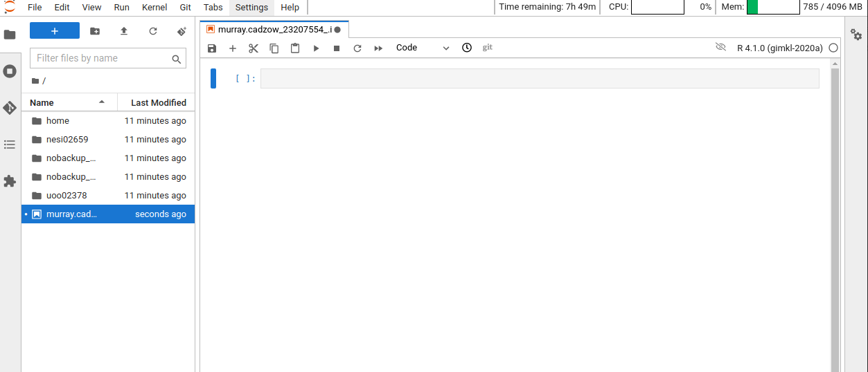
After logging into the NeSI Jupyter lab, open an R (v4.1) notebook.
Now that we are ready to start exploring R, we will want to keep a record of the commands we are using in out notebook. Lets first save our new notebook.
Click the File menu and select Save Notebook As and then call it
intro_r.ipynb. By convention, notebooks end with the file extension .ipynb.
Overview of the R notebook layout
Here are the main features of the notebook environment:
Some useful keyboard shortcuts:
- To run the current cell: Shift + ENTER
- To insert a new cell above the current cell: ESC + A
- To insert a new cell below the current cell: ESC + B
You are working with R
Although we won’t be working with R at the terminal, there are lots of reasons to. For example, once you have written an RScript, you can run it at any Linux or Windows terminal without the need to start up RStudio. We don’t want you to get confused - Jupyter or RStudio runs R, but R is not RStudio or Jupyter. For more on running an R Script at the terminal see this Software Carpentry lesson.
Getting to work with R: navigating directories
Now that we have covered the more aesthetic aspects of Jupyter notebooks, we can get to work using some commands. We will write, execute, and save the commands we learn in our notebook. First, lets see what directory we are in. To do so, type the following command into the cell:
getwd()
To execute this command, make sure your cursor is on the same line the command is written. Then click the Run (play) button that is just above the first line of your notebook in the header.
In the output, we expect to see the following output*:
[1] "'/scale_wlg_persistent/filesets/home/murray.cadzow/.jupyter/jobs/23207554'"
Since we will be learning several commands, we may already want to keep some
short notes in our notebook to explain the purpose of the command. Entering a #
before any line in a cell turns that line into a comment, which R will
not try to interpret as code. Edit your cell to include a comment on the
purpose of commands you are learning, e.g.:
# this command shows the current working directory
getwd()
Exercise: Work interactively in R
What happens when you try to enter the
getwd()command in the Console pane?Solution
You will get the same output you did as when you ran
getwd()from the source. You can run any command in the Console, however, executing it from the source script will make it easier for us to record what we have done, and ultimately run an entire script, instead of entering commands one-by-one.
For the purposes of this exercise we want you to be in the directory "~/obss_2021/intro_r".
What if you weren’t? You can set your home directory using the setwd()
command. Enter this command in your script, but don’t run this yet.
# This sets the working directory
setwd()
You may have guessed, you need to tell the setwd() command
what directory you want to set as your working directory. To do so, inside of
the parentheses, open a set of quotes. Inside the quotes enter a ~/ which is
your home directory for Linux. Next, use the Tab key, to take
advantage of the Tab-autocompletion method, to select obss_2021, and intro_r directory. The path in your script should look like this:
# This sets the working directory
setwd("~/obss_2021/intro_r")
When you run this command, the console repeats the command, but gives you no
output. Instead, you see the blank R prompt: >. Congratulations! Although it
seems small, knowing what your working directory is and being able to set your
working directory is the first step to analyzing your data.
Tip: Never use
setwd()Wait, what was the last 2 minutes about? Well, if setting your working directory is something you need to do, you need to be very careful about using this as a step in your script. For example, what if your script is being on a computer that has a different directory structure? The top-level path in a Unix file system is root
/, but on Windows it is likelyC:\. This is one of several ways you might cause a script to break because a file path is configured differently than your script anticipates. R packages like here and file.path allow you to specify file paths is a way that is more operating system independent. See Jenny Bryan’s blog post for this and other R tips.
Using functions in R, without needing to master them
A function in R (or any computing language) is a short
program that takes some input and returns some output. Functions may seem like an advanced topic (and they are), but you have already
used at least one function in R. getwd() is a function! The next sections will help you understand what is happening in
any R script.
Exercise: What do these functions do?
Try the following functions by writing them in your script. See if you can guess what they do, and make sure to add comments to your script about your assumed purpose.
dir()sessionInfo()date()Sys.time()Solution
dir()# Lists files in the working directorysessionInfo()# Gives the version of R and additional info including on attached packagesdate()# Gives the current dateSys.time()# Gives the current timeNotice: Commands are case sensitive!
You have hopefully noticed a pattern - an R function has three key properties:
- Functions have a name (e.g.
dir,getwd); note that functions are case sensitive! - Following the name, functions have a pair of
() - Inside the parentheses, a function may take 0 or more arguments
An argument may be a specific input for your function and/or may modify the
function’s behavior. For example the function round() will round a number
with a decimal:
# This will round a number to the nearest integer
round(3.14)
[1] 3
Getting help with function arguments
What if you wanted to round to one significant digit? round() can
do this, but you may first need to read the help to find out how. To see the help
(In R sometimes also called a “vignette”) enter a ? in front of the function
name:
?round()
The “Help” tab will show you information (often, too much information). You
will slowly learn how to read and make sense of help files. Checking the “Usage” or “Examples”
headings is often a good place to look first. If you look under “Arguments,” we
also see what arguments we can pass to this function to modify its behavior.
You can also see a function’s argument using the args() function:
args(round)
function (x, digits = 0)
NULL
round() takes two arguments, x, which is the number to be
rounded, and a
digits argument. The = sign indicates that a default (in this case 0) is
already set. Since x is not set, round() requires we provide it, in contrast
to digits where R will use the default value 0 unless you explicitly provide
a different value. We can explicitly set the digits parameter when we call the
function:
round(3.14159, digits = 2)
[1] 3.14
Or, R accepts what we call “positional arguments”, if you pass a function
arguments separated by commas, R assumes that they are in the order you saw
when we used args(). In the case below that means that x is 3.14159 and
digits is 2.
round(3.14159, 2)
[1] 3.14
Finally, what if you are using ? to get help for a function in a package not installed on your system, such as when you are running a script which has dependencies.
?geom_point()
will return an error:
Error in .helpForCall(topicExpr, parent.frame()) :
   no methods for ‘geom_point’ and no documentation for it as a function
Use two question marks (i.e. ??geom_point()) and R will return
results from a search of the documentation for packages you have installed on your computer
in the “Help” tab. Finally, if you think there
should be a function, for example a statistical test, but you aren’t
sure what it is called in R, or what functions may be available, use
the help.search() function.
Exercise: Searching for R functions
Use
help.search()to find R functions for the following statistical functions. Remember to put your search query in quotes inside the function’s parentheses.
- Chi-Squared test
- Student t-test
- mixed linear model
Solution
While your search results may return several tests, we list a few you might find:
- Chi-Squared test:
stats::Chisquare- Student t-test:
stats::t.test- mixed linear model:
stats::lm.glm
We will discuss more on where to look for the libraries and packages that contain functions you want to use. For now, be aware that two important ones are CRAN - the main repository for R, and Bioconductor - a popular repository for bioinformatics-related R packages.
Key Points
R is a powerful, popular open-source scripting language
R Basics
Overview
Teaching: 60 min
Exercises: 20 minQuestions
What will these lessons not cover?
What are the basic features of the R language?
What are the most common objects in R?
Objectives
Be able to create the most common R objects including vectors
Understand that vectors have modes, which correspond to the type of data they contain
Be able to use arithmetic operators on R objects
Be able to retrieve (subset), name, or replace, values from a vector
Be able to use logical operators in a subsetting operation
Understand that lists can hold data of more than one mode and can be indexed
This lesson has been adapted from https://datacarpentry.org/genomics-r-intro/02-r-basics/index.html
“The fantastic world of R awaits you” OR “Nobody wants to learn how to use R”
Before we begin this lesson, we want you to be clear on the goal of the workshop and these lessons. We believe that every learner can achieve competency with R. You have reached competency when you find that you are able to use R to handle common analysis challenges in a reasonable amount of time (which includes time needed to look at learning materials, search for answers online, and ask colleagues for help). As you spend more time using R (there is no substitute for regular use and practice) you will find yourself gaining competency and even expertise. The more familiar you get, the more complex the analyses you will be able to carry out, with less frustration, and in less time - the fantastic world of R awaits you!
What these lessons will not teach you
Nobody wants to learn how to use R. People want to learn how to use R to analyze their own research questions! Ok, maybe some folks learn R for R’s sake, but these lessons assume that you want to start analyzing genomic data as soon as possible. Given this, there are many valuable pieces of information about R that we simply won’t have time to cover. Hopefully, we will clear the hurdle of giving you just enough knowledge to be dangerous, which can be a high bar in R! We suggest you look into the additional learning materials in the tip box below.
Here are some R skills we will not cover in these lessons
- How to create and work with R matrices and R lists
- How to create and work with loops and conditional statements, and the “apply” family of functions (which are super useful, read more here)
- How to do basic string manipulations (e.g. finding patterns in text using grep, replacing text)
- How to plot using the default R graphic tools
- How to use advanced R statistical functions
Tip: Where to learn more
The following are good resources for learning more about R. Some of them can be quite technical, but if you are a regular R user you may ultimately need this technical knowledge.
- R for Beginners: By Emmanuel Paradis and a great starting point
- The R Manuals: Maintained by the R project
- R contributed documentation: Also linked to the R project; importantly there are materials available in several languages
- R for Data Science: A wonderful collection by noted R educators and developers Garrett Grolemund and Hadley Wickham
- Practical Data Science for Stats: Not exclusively about R usage, but a nice collection of pre-prints on data science and applications for R
- Programming in R Software Carpentry lesson: There are several Software Carpentry lessons in R to choose from
Creating objects in R
Reminder
At this point you should be coding along in your notebook we created in the last episode. Writing your commands in the notebook (and commenting it) will make it easier to record what you did and why.
What might be called a variable in many languages is called an object in R.
To create an object you need:
- a name (e.g. ‘a’)
- a value (e.g. ‘1’)
- the assignment operator (‘<-‘)
In your script, “genomics_r_basics.R”, using the R assignment operator ‘<-‘, assign ‘1’ to the object ‘a’ as shown. Remember to leave a comment in the line above (using the ‘#’) to explain what you are doing:
# this line creates the object 'a' and assigns it the value '1'

a <- 1
Next, run this line of code in your script. You can run a line of code by hitting the Run button that is just above the first line of your notebook in the header of the pane or you can use the appropriate shortcut:
- execution shortcut: Shift+Enter
Beneath the cell you should see a new cell appear. There won’t be any output shown but there will now be an object called a in our environment.
To see what objects are in the environment we can use the ls() function.
# this line tells us the objects in the environment

ls()
'a'
If we cant to get back the value stored in an object we use its name
# this line outputs the value stored in the object called 'a'

a
[1] 1
Exercise: Create some objects in R
Create the following objects; give each object an appropriate name (your best guess at what name to use is fine):
- Create an object that has the value of number of pairs of human chromosomes
- Create an object that has a value of your favorite gene name
- Create an object that has this URL as its value: “ftp://ftp.ensemblgenomes.org/pub/bacteria/release-39/fasta/bacteria_5_collection/escherichia_coli_b_str_rel606/”
- Create an object that has the value of the number of chromosomes in a diploid human cell
Solution
Here as some possible answers to the challenge:
human_chr_number <- 23
gene_name <- 'pten'
ensemble_url <- 'ftp://ftp.ensemblgenomes.org/pub/bacteria/release-39/fasta/bacteria_5_collection/escherichia_coli_b_str_rel606/'
human_diploid_chr_num <-  2 * human_chr_number
Naming objects in R
Here are some important details about naming objects in R.
- Avoid spaces and special characters: Object names cannot contain spaces or the minus sign (
-). You can use ‘_’ to make names more readable. You should avoid using special characters in your object name (e.g. ! @ # . , etc.). Also, object names cannot begin with a number. - Use short, easy-to-understand names: You should avoid naming your objects using single letters (e.g. ‘n’, ‘p’, etc.). This is mostly to encourage you to use names that would make sense to anyone reading your code (a colleague, or even yourself a year from now). Also, avoiding excessively long names will make your code more readable.
- Avoid commonly used names: There are several names that may already have a definition in the R language (e.g. ‘mean’, ‘min’, ‘max’). One clue that a name already has meaning is that if you start typing a name in RStudio and it gets a colored highlight or RStudio gives you a suggested autocompletion you have chosen a name that has a reserved meaning.
- Use the recommended assignment operator: In R, we use ‘<- ‘ as the preferred assignment operator. ‘=’ works too, but is most commonly used in passing arguments to functions (more on functions later).
There are a few more suggestions about naming and style you may want to learn more about as you write more R code. There are several “style guides” that have advice, and one to start with is the tidyverse R style guide.
Tip: Pay attention to warnings in the output
If you enter a line of code in your notebook that contains an error, Jupyter may give you an error message and underline this mistake. Sometimes these messages are easy to understand, but often the messages may need some figuring out. Paying attention to these warnings will help you avoid mistakes. In the example below, our object name has a space, which is not allowed in R. The error message does not say this directly, but R is “not sure” about how to assign the name to “human_ chr_number” when the object name we want is “human_chr_number”.

Reassigning object names or deleting objects
Once an object has a value, you can change that value by overwriting it. R will not give you a warning or error if you overwriting an object, which may or may not be a good thing depending on how you look at it.
# gene_name has the value 'pten' or whatever value you used in the challenge.
# We will now assign the new value 'tp53'
gene_name <- 'tp53'
You can also remove an object from R’s memory entirely. The rm() function
will delete the object.
# delete the object 'gene_name'
rm(gene_name)
If you run a line of code that has only an object name, R will normally display the contents of that object. In this case, we are told the object no longer exists.
Error: object 'gene_name' not found
Understanding object data types (modes)
In R, every object has two properties:
- Length: How many distinct values are held in that object
- Mode: What is the classification (type) of that object.
We will get to the “length” property later in the lesson. The “mode” property corresponds to the type of data an object represents. The most common modes you will encounter in R are:
| Mode (abbreviation) | Type of data |
|---|---|
| Numeric (num) | Numbers such floating point/decimals (1.0, 0.5, 3.14), there are also more specific numeric types (dbl - Double, int - Integer). These differences are not relevant for most beginners and pertain to how these values are stored in memory |
| Character (chr) | A sequence of letters/numbers in single ‘’ or double “ “ quotes |
| Logical | Boolean values - TRUE or FALSE |
There are a few other modes (i.e. “complex”, “raw” etc.) but these are the three we will work with in this lesson.
Data types are familiar in many programming languages, but also in natural language where we refer to them as the parts of speech, e.g. nouns, verbs, adverbs, etc. Once you know if a word - perhaps an unfamiliar one - is a noun, you can probably guess you can count it and make it plural if there is more than one (e.g. 1 Tuatara, or 2 Tuataras). If something is a adjective, you can usually change it into an adverb by adding “-ly” (e.g. jejune vs. jejunely). Depending on the context, you may need to decide if a word is in one category or another (e.g “cut” may be a noun when it’s on your finger, or a verb when you are preparing vegetables). These concepts have important analogies when working with R objects.
Exercise: Create objects and check their modes
Create the following objects in R, then use the
mode()function to verify their modes. Try to guess what the mode will be before you look at the solution
chromosome_name <- 'chr02'od_600_value <- 0.47chr_position <- '1001701'spock <- TRUEpilot <- EarhartSolution
Error in eval(expr, envir, enclos): object 'Earhart' not foundmode(chromosome_name)[1] "character"mode(od_600_value)[1] "numeric"mode(chr_position)[1] "character"mode(spock)[1] "logical"mode(pilot)Error in mode(pilot): object 'pilot' not found
Notice from the solution that even if a series of numbers is given as a value
R will consider them to be in the “character” mode if they are enclosed as
single or double quotes. Also, notice that you cannot take a string of alphanumeric
characters (e.g. Earhart) and assign as a value for an object. In this case,
R looks for an object named Earhart but since there is no object, no assignment can
be made. If Earhart did exist, then the mode of pilot would be whatever
the mode of Earhart was originally. If we want to create an object
called pilot that was the name “Earhart”, we need to enclose
Earhart in quotation marks.
pilot <- "Earhart"
mode(pilot)
[1] "character"
Mathematical and functional operations on objects
Once an object exists (which by definition also means it has a mode), R can appropriately manipulate that object. For example, objects of the numeric modes can be added, multiplied, divided, etc. R provides several mathematical (arithmetic) operators including:
| Operator | Description |
|---|---|
| + | addition |
| - | subtraction |
| * | multiplication |
| / | division |
| ^ or ** | exponentiation |
| a%/%b | integer division (division where the remainder is discarded) |
| a%%b | modulus (returns the remainder after division) |
These can be used with literal numbers:
(1 + (5 ** 0.5))/2
[1] 1.618034
and importantly, can be used on any object that evaluates to (i.e. interpreted by R) a numeric object:
# multiply the object 'human_chr_number' by 2

human_chr_number * 2
[1] 46
Exercise: Compute the golden ratio
One approximation of the golden ratio (φ) can be found by taking the sum of 1 and the square root of 5, and dividing by 2 as in the example above. Compute the golden ratio to 3 digits of precision using the
sqrt()andround()functions. Hint: remember theround()function can take 2 arguments.Solution
round((1 + sqrt(5))/2, digits = 3)[1] 1.618Notice that you can place one function inside of another.
Vectors
Vectors are probably the
most used commonly used object type in R.
A vector is a collection of values that are all of the same type (numbers, characters, etc.).
One of the most common
ways to create a vector is to use the c() function - the “concatenate” or
“combine” function. Inside the function you may enter one or more values; for
multiple values, separate each value with a comma:
# Create the SNP gene name vector

snp_genes <- c("OXTR", "ACTN3", "AR", "OPRM1")
Vectors always have a mode and a length.
You can check these with the mode() and length() functions respectively.
Another useful function that gives both of these pieces of information is the
str() (structure) function.
# Check the mode, length, and structure of 'snp_genes'
mode(snp_genes)
[1] "character"
length(snp_genes)
[1] 4
str(snp_genes)
chr [1:4] "OXTR" "ACTN3" "AR" "OPRM1"
Vectors are quite important in R. Another data type that we will work with later in this lesson, data frames, are collections of vectors. What we learn here about vectors will pay off even more when we start working with data frames.
Creating and subsetting vectors
Let’s create a few more vectors to play around with:
# Some interesting human SNPs
# while accuracy is important, typos in the data won't hurt you here

snps <- c('rs53576', 'rs1815739', 'rs6152', 'rs1799971')
snp_chromosomes <- c('3', '11', 'X', '6')
snp_positions <- c(8762685, 66560624, 67545785, 154039662)
Once we have vectors, one thing we may want to do is specifically retrieve one or more values from our vector. To do so, we use bracket notation. We type the name of the vector followed by square brackets. In those square brackets we place the index (e.g. a number) in that bracket as follows:
# get the 3rd value in the snp_genes vector
snp_genes[3]
[1] "AR"
In R, every item your vector is indexed, starting from the first item (1) through to the final number of items in your vector. You can also retrieve a range of numbers:
# get the 1st through 3rd value in the snp_genes vector

snp_genes[1:3]
[1] "OXTR" "ACTN3" "AR"
If you want to retrieve several (but not necessarily sequential) items from a vector, you pass a vector of indices; a vector that has the numbered positions you wish to retrieve.
# get the 1st, 3rd, and 4th value in the snp_genes vector

snp_genes[c(1, 3, 4)]
[1] "OXTR" "AR" "OPRM1"
There are additional (and perhaps less commonly used) ways of subsetting a vector (see these examples). Also, several of these subsetting expressions can be combined:
# get the 1st through the 3rd value, and 4th value in the snp_genes vector
# yes, this is a little silly in a vector of only 4 values.
snp_genes[c(1:3,4)]
[1] "OXTR" "ACTN3" "AR" "OPRM1"
Adding to, removing, or replacing values in existing vectors
Once you have an existing vector, you may want to add a new item to it. To do
so, you can use the c() function again to add your new value:
# add the gene 'CYP1A1' and 'APOA5' to our list of snp genes
# this overwrites our existing vector
snp_genes <- c(snp_genes, "CYP1A1", "APOA5")
We can verify that “snp_genes” contains the new gene entry
snp_genes
[1] "OXTR" "ACTN3" "AR" "OPRM1" "CYP1A1" "APOA5"
Using a negative index will return a version of a vector with that index’s value removed:
snp_genes[-6]
[1] "OXTR" "ACTN3" "AR" "OPRM1" "CYP1A1"
We can remove that value from our vector by overwriting it with this expression:
snp_genes <- snp_genes[-6]
snp_genes
[1] "OXTR" "ACTN3" "AR" "OPRM1" "CYP1A1"
We can also explicitly rename or add a value to our index using double bracket notation:
snp_genes[7]<- "APOA5"
snp_genes
[1] "OXTR" "ACTN3" "AR" "OPRM1" "CYP1A1" NA "APOA5"
Notice in the operation above that R inserts an NA value to extend our vector so that the gene “APOA5” is an index 7. This may be a good or not-so-good thing depending on how you use this.
Exercise: Examining and subsetting vectors
Answer the following questions to test your knowledge of vectors
Which of the following are true of vectors in R? A) All vectors have a mode or a length
B) All vectors have a mode and a length
C) Vectors may have different lengths
D) Items within a vector may be of different modes
E) You can use thec()to add one or more items to an existing vector
F) You can use thec()to add a vector to an exiting vectorSolution
A) False - Vectors have both of these properties
B) True
C) True
D) False - Vectors have only one mode (e.g. numeric, character); all items in
a vector must be of this mode. E) True
F) True
Logical Subsetting
There is one last set of cool subsetting capabilities we want to introduce. It is possible within R to retrieve items in a vector based on a logical evaluation or numerical comparison. For example, let’s say we wanted get all of the SNPs in our vector of SNP positions that were greater than 100,000,000. We could index using the ‘>’ (greater than) logical operator:
snp_positions[snp_positions > 100000000]
[1] 154039662
In the square brackets you place the name of the vector followed by the comparison operator and (in this case) a numeric value. Some of the most common logical operators you will use in R are:
| Operator | Description |
|---|---|
| < | less than |
| <= | less than or equal to |
| > | greater than |
| >= | greater than or equal to |
| == | exactly equal to |
| != | not equal to |
| !x | not x |
| a | b | a or b |
| a & b | a and b |
The magic of programming
The reason why the expression
snp_positions[snp_positions > 100000000]works can be better understood if you examine what the expression “snp_positions > 100000000” evaluates to:snp_positions > 100000000[1] FALSE FALSE FALSE TRUEThe output above is a logical vector, the 4th element of which is TRUE. When you pass a logical vector as an index, R will return the true values:
snp_positions[c(FALSE, FALSE, FALSE, TRUE)][1] 154039662If you have never coded before, this type of situation starts to expose the “magic” of programming. We mentioned before that in the bracket notation you take your named vector followed by brackets which contain an index: named_vector[index]. The “magic” is that the index needs to evaluate to a number. So, even if it does not appear to be an integer (e.g. 1, 2, 3), as long as R can evaluate it, we will get a result. That our expression
snp_positions[snp_positions > 100000000]evaluates to a number can be seen in the following situation. If you wanted to know which index (1, 2, 3, or 4) in our vector of SNP positions was the one that was greater than 100,000,000?We can use the
which()function to return the indices of any item that evaluates as TRUE in our comparison:which(snp_positions > 100000000)[1] 4Why this is important
Often in programming we will not know what inputs and values will be used when our code is executed. Rather than put in a pre-determined value (e.g 100000000) we can use an object that can take on whatever value we need. So for example:
snp_marker_cutoff <- 100000000
snp_positions[snp_positions > snp_marker_cutoff]
[1] 154039662Ultimately, it’s putting together flexible, reusable code like this that gets at the “magic” of programming!
A few final vector tricks
Finally, there are a few other common retrieve or replace operations you may
want to know about. First, you can check to see if any of the values of your
vector are missing (i.e. are NA). Missing data will get a more detailed treatment later,
but the is.NA() function will return a logical vector, with TRUE for any NA
value:
# current value of 'snp_genes':
# chr [1:7] "OXTR" "ACTN3" "AR" "OPRM1" "CYP1A1" NA "APOA5"

is.na(snp_genes)
[1] FALSE FALSE FALSE FALSE FALSE TRUE FALSE
Sometimes, you may wish to find out if a specific value (or several values) is
present a vector. You can do this using the comparison operator %in%, which
will return TRUE for any value in your collection that is in
the vector you are searching:
# current value of 'snp_genes':
# chr [1:7] "OXTR" "ACTN3" "AR" "OPRM1" "CYP1A1" NA "APOA5"

# test to see if "ACTN3" or "APO5A" is in the snp_genes vector
# if you are looking for more than one value, you must pass this as a vector

c("ACTN3","APOA5") %in% snp_genes
[1] TRUE TRUE
Review Exercise 1
What data types/modes are the following vectors? a.
snps
b.snp_chromosomes
c.snp_positionsSolution
typeof(snps)[1] "character"typeof(snp_chromosomes)[1] "character"typeof(snp_positions)[1] "double"
Review Exercise 2
Add the following values to the specified vectors: a. To the
snpsvector add: ‘rs662799’
b. To thesnp_chromosomesvector add: 11
c. To thesnp_positionsvector add: 116792991Solution
snps <- c(snps, 'rs662799')
snps
[1] "rs53576" "rs1815739" "rs6152" "rs1799971" "rs662799"snp_chromosomes <- c(snp_chromosomes, "11") # did you use quotes? snp_chromosomes[1] "3" "11" "X" "6" "11"snp_positions <- c(snp_positions, 116792991) snp_positions[1] 8762685 66560624 67545785 154039662 116792991
Review Exercise 3
Make the following change to the
snp_genesvector:Hint: Your vector should look like this in ‘Environment’:
chr [1:7] "OXTR" "ACTN3" "AR" "OPRM1" "CYP1A1" NA "APOA5". If not recreate the vector by running this expression:snp_genes <- c("OXTR", "ACTN3", "AR", "OPRM1", "CYP1A1", NA, "APOA5")a. Create a new version of
snp_genesthat does not contain CYP1A1 and then
b. Add 2 NA values to the end ofsnp_genesSolution
snp_genes <- snp_genes[-5]
snp_genes <- c(snp_genes, NA, NA)
snp_genes
[1] "OXTR" "ACTN3" "AR" "OPRM1" NA "APOA5" NA NA
Review Exercise 4
Using indexing, create a new vector named
combinedthat contains:
- The the 1st value in
snp_genes- The 1st value in
snps- The 1st value in
snp_chromosomes- The 1st value in
snp_positionsSolution
combined <- c(snp_genes[1], snps[1], snp_chromosomes[1], snp_positions[1])
combined
[1] "OXTR" "rs53576" "3" "8762685"
Review Exercise 5
What type of data is
combined?Solution
typeof(combined)[1] "character"
Bonus material: Lists
Lists are quite useful in R, but we won’t be using them in the genomics lessons. That said, you may come across lists in the way that some bioinformatics programs may store and/or return data to you. One of the key attributes of a list is that, unlike a vector, a list may contain data of more than one mode. Learn more about creating and using lists using this nice tutorial. In this one example, we will create a named list and show you how to retrieve items from the list.
# Create a named list using the 'list' function and our SNP examples
# Note, for easy reading we have placed each item in the list on a separate line
# Nothing special about this, you can do this for any multiline commands
# To run this command, make sure the entire command (all 4 lines) are highlighted
# before running
# Note also, as we are doing all this inside the list() function use of the
# '=' sign is good style
snp_data <- list(genes = snp_genes,
                 refference_snp = snps,
                 chromosome = snp_chromosomes,
                 position = snp_positions)
# Examine the structure of the list
str(snp_data)
List of 4
 $ genes         : chr [1:8] "OXTR" "ACTN3" "AR" "OPRM1" ...
 $ refference_snp: chr [1:5] "rs53576" "rs1815739" "rs6152" "rs1799971" ...
 $ chromosome    : chr [1:5] "3" "11" "X" "6" ...
 $ position      : num [1:5] 8.76e+06 6.66e+07 6.75e+07 1.54e+08 1.17e+08
To get all the values for the position object in the list, we use the $ notation:
# return all the values of position object

snp_data$position
[1] 8762685 66560624 67545785 154039662 116792991
To get the first value in the position object, use the [] notation to index:
# return first value of the position object

snp_data$position[1]
[1] 8762685
Key Points
Effectively using R is a journey of months or years. Still you don’t have to be an expert to use R and you can start using and analyzing your data with with about a day’s worth of training
It is important to understand how data are organized by R in a given object type and how the mode of that type (e.g. numeric, character, logical, etc.) will determine how R will operate on that data.
Working with vectors effectively prepares you for understanding how data are organized in R.
R Basics continued - factors and data frames
Overview
Teaching: 60 min
Exercises: 30 minQuestions
How do I get started with tabular data (e.g. spreadsheets) in R?
What are some best practices for reading data into R?
How do I save tabular data generated in R?
Objectives
Explain the basic principle of tidy datasets
Be able to load a tabular dataset using base R functions
Be able to determine the structure of a data frame including its dimensions and the datatypes of variables
Be able to subset/retrieve values from a data frame
Understand how R may coerce data into different modes
Be able to change the mode of an object
Understand that R uses factors to store and manipulate categorical data
Be able to manipulate a factor, including subsetting and reordering
Be able to apply an arithmetic function to a data frame
Be able to coerce the class of an object (including variables in a data frame)
Be able to import data from Excel
Be able to save a data frame as a delimited file
** This lesson was adapted from https://datacarpentry.org/genomics-r-intro/03-basics-factors-dataframes/index.html**
Working with spreadsheets (tabular data)
A substantial amount of the data we work with in genomics will be tabular data, this is data arranged in rows and columns - also known as spreadsheets. We could write a whole lesson on how to work with spreadsheets effectively (actually we did). For our purposes, we want to remind you of a few principles before we work with our first set of example data:
1) Keep raw data separate from analyzed data
This is principle number one because if you can’t tell which files are the original raw data, you risk making some serious mistakes (e.g. drawing conclusion from data which have been manipulated in some unknown way).
2) Keep spreadsheet data Tidy
The simplest principle of Tidy data is that we have one row in our spreadsheet for each observation or sample, and one column for every variable that we measure or report on. As simple as this sounds, it’s very easily violated. Most data scientists agree that significant amounts of their time is spent tidying data for analysis. Read more about data organization in our lesson and in this paper.
3) Trust but verify
Finally, while you don’t need to be paranoid about data, you should have a plan for how you will prepare it for analysis. This a focus of this lesson. You probably already have a lot of intuition, expectations, assumptions about your data - the range of values you expect, how many values should have been recorded, etc. Of course, as the data get larger our human ability to keep track will start to fail (and yes, it can fail for small data sets too). R will help you to examine your data so that you can have greater confidence in your analysis, and its reproducibility.
Tip: Keeping you raw data separate
When you work with data in R, you are not changing the original file you loaded that data from. This is different than (for example) working with a spreadsheet program where changing the value of the cell leaves you one “save”-click away from overwriting the original file. You have to purposely use a writing function (e.g.
write.csv()) to save data loaded into R. In that case, be sure to save the manipulated data into a new file. More on this later in the lesson.
Importing tabular data into R
There are several ways to import data into R. For our purpose here, we will
focus on using the tools every R installation comes with (so called “base” R) to
import a comma-delimited file containing the results of our variant calling workflow.
We will need to load the sheet using a function called read.csv().
Exercise: Review the arguments of the
read.csv()functionBefore using the
read.csv()function, use R’s help feature to answer the following questions.Hint: Entering ‘?’ before the function name and then running that line will bring up the help documentation. Also, when reading this particular help be careful to pay attention to the ‘read.csv’ expression under the ‘Usage’ heading. Other answers will be in the ‘Arguments’ heading.
A) What is the default parameter for ‘header’ in the
read.csv()function?B) What argument would you have to change to read a file that was delimited by semicolons (;) rather than commas?
C) What argument would you have to change to read file in which numbers used commas for decimal separation (i.e. 1,00)?
D) What argument would you have to change to read in only the first 10,000 rows of a very large file?
Solution
A) The
read.csv()function has the argument ‘header’ set to TRUE by default, this means the function always assumes the first row is header information, (i.e. column names)B) The
read.csv()function has the argument ‘sep’ set to “,”. This means the function assumes commas are used as delimiters, as you would expect. Changing this parameter (e.g.sep=";") would now interpret semicolons as delimiters.C) Although it is not listed in the
read.csv()usage,read.csv()is a “version” of the functionread.table()and accepts all its arguments. If you setdec=","you could change the decimal operator. We’d probably assume the delimiter is some other character.D) You can set
nrowto a numeric value (e.g.nrow=10000) to choose how many rows of a file you read in. This may be useful for very large files where not all the data is needed to test some data cleaning steps you are applying.Hopefully, this exercise gets you thinking about using the provided help documentation in R. There are many arguments that exist, but which we wont have time to cover. Look here to get familiar with functions you use frequently, you may be surprised at what you find they can do.
Now, let’s read in the file combined_tidy_vcf.csv which will be located in
~/obss_2021/intro_r/. Call this data variants. The
first argument to pass to our read.csv() function is the file path for our
data. The file path must be in quotes and now is a good time to remember to
use tab autocompletion. If you use tab autocompletion you avoid typos and
errors in file paths. Use it!
## read in a CSV file and save it as 'variants'

variants <- read.csv("~/obss_2021/intro_r/combined_tidy_vcf.csv")
Lets use str() to get an idea of what we’re dealing with.
# Find out the names, datatypes, and dimensions

str(variants)
'data.frame':	801 obs. of  29 variables:
 $ sample_id    : chr  "SRR2584863" "SRR2584863" "SRR2584863" "SRR2584863" ...
 $ CHROM        : chr  "CP000819.1" "CP000819.1" "CP000819.1" "CP000819.1" ...
 $ POS          : int  9972 263235 281923 433359 473901 648692 1331794 1733343 2103887 2333538 ...
 $ ID           : logi  NA NA NA NA NA NA ...
 $ REF          : chr  "T" "G" "G" "CTTTTTTT" ...
 $ ALT          : chr  "G" "T" "T" "CTTTTTTTT" ...
 $ QUAL         : num  91 85 217 64 228 210 178 225 56 167 ...
 $ FILTER       : logi  NA NA NA NA NA NA ...
 $ INDEL        : logi  FALSE FALSE FALSE TRUE TRUE FALSE ...
 $ IDV          : int  NA NA NA 12 9 NA NA NA 2 7 ...
 $ IMF          : num  NA NA NA 1 0.9 ...
 $ DP           : int  4 6 10 12 10 10 8 11 3 7 ...
 $ VDB          : num  0.0257 0.0961 0.7741 0.4777 0.6595 ...
 $ RPB          : num  NA 1 NA NA NA NA NA NA NA NA ...
 $ MQB          : num  NA 1 NA NA NA NA NA NA NA NA ...
 $ BQB          : num  NA 1 NA NA NA NA NA NA NA NA ...
 $ MQSB         : num  NA NA 0.975 1 0.916 ...
 $ SGB          : num  -0.556 -0.591 -0.662 -0.676 -0.662 ...
 $ MQ0F         : num  0 0.167 0 0 0 ...
 $ ICB          : logi  NA NA NA NA NA NA ...
 $ HOB          : logi  NA NA NA NA NA NA ...
 $ AC           : int  1 1 1 1 1 1 1 1 1 1 ...
 $ AN           : int  1 1 1 1 1 1 1 1 1 1 ...
 $ DP4          : chr  "0,0,0,4" "0,1,0,5" "0,0,4,5" "0,1,3,8" ...
 $ MQ           : int  60 33 60 60 60 60 60 60 60 60 ...
 $ Indiv        : chr  "/home/dcuser/dc_workshop/results/bam/SRR2584863.aligned.sorted.bam" "/home/dcuser/dc_workshop/results/bam/SRR2584863.aligned.sorted.bam" "/home/dcuser/dc_workshop/results/bam/SRR2584863.aligned.sorted.bam" "/home/dcuser/dc_workshop/results/bam/SRR2584863.aligned.sorted.bam" ...
 $ gt_PL        : chr  "121,0" "112,0" "247,0" "91,0" ...
 $ gt_GT        : int  1 1 1 1 1 1 1 1 1 1 ...
 $ gt_GT_alleles: chr  "G" "T" "T" "CTTTTTTTT" ...
Summarizing, subsetting, and determining the structure of a data frame.
A data frame is the standard way in R to store tabular data. A data fame could also be thought of as a collection of vectors, all of which have the same length. Using only two functions, we can learn a lot about out data frame including some summary statistics as well as well as the “structure” of the data frame. Let’s examine what each of these functions can tell us:
## get summary statistics on a data frame

summary(variants)
  sample_id            CHROM                POS             ID
 Length:801         Length:801         Min.   :   1521   Mode:logical
 Class :character   Class :character   1st Qu.:1115970   NA's:801
 Mode  :character   Mode  :character   Median :2290361
                                       Mean   :2243682
                                       3rd Qu.:3317082
                                       Max.   :4629225

     REF                ALT                 QUAL          FILTER
 Length:801         Length:801         Min.   :  4.385   Mode:logical
 Class :character   Class :character   1st Qu.:139.000   NA's:801
 Mode  :character   Mode  :character   Median :195.000
                                       Mean   :172.276
                                       3rd Qu.:225.000
                                       Max.   :228.000

   INDEL              IDV              IMF               DP
 Mode :logical   Min.   : 2.000   Min.   :0.5714   Min.   : 2.00
 FALSE:700       1st Qu.: 7.000   1st Qu.:0.8824   1st Qu.: 7.00
 TRUE :101       Median : 9.000   Median :1.0000   Median :10.00
                 Mean   : 9.396   Mean   :0.9219   Mean   :10.57
                 3rd Qu.:11.000   3rd Qu.:1.0000   3rd Qu.:13.00
                 Max.   :20.000   Max.   :1.0000   Max.   :79.00
                 NA's   :700      NA's   :700
      VDB                 RPB              MQB              BQB
 Min.   :0.0005387   Min.   :0.0000   Min.   :0.0000   Min.   :0.1153
 1st Qu.:0.2180410   1st Qu.:0.3776   1st Qu.:0.1070   1st Qu.:0.6963
 Median :0.4827410   Median :0.8663   Median :0.2872   Median :0.8615
 Mean   :0.4926291   Mean   :0.6970   Mean   :0.5330   Mean   :0.7784
 3rd Qu.:0.7598940   3rd Qu.:1.0000   3rd Qu.:1.0000   3rd Qu.:1.0000
 Max.   :0.9997130   Max.   :1.0000   Max.   :1.0000   Max.   :1.0000
                     NA's   :773      NA's   :773      NA's   :773
      MQSB              SGB               MQ0F           ICB
 Min.   :0.01348   Min.   :-0.6931   Min.   :0.00000   Mode:logical
 1st Qu.:0.95494   1st Qu.:-0.6762   1st Qu.:0.00000   NA's:801
 Median :1.00000   Median :-0.6620   Median :0.00000
 Mean   :0.96428   Mean   :-0.6444   Mean   :0.01127
 3rd Qu.:1.00000   3rd Qu.:-0.6364   3rd Qu.:0.00000
 Max.   :1.01283   Max.   :-0.4536   Max.   :0.66667
 NA's   :48
   HOB                AC          AN        DP4                  MQ
 Mode:logical   Min.   :1   Min.   :1   Length:801         Min.   :10.00
 NA's:801       1st Qu.:1   1st Qu.:1   Class :character   1st Qu.:60.00
                Median :1   Median :1   Mode  :character   Median :60.00
                Mean   :1   Mean   :1                      Mean   :58.19
                3rd Qu.:1   3rd Qu.:1                      3rd Qu.:60.00
                Max.   :1   Max.   :1                      Max.   :60.00

    Indiv              gt_PL               gt_GT   gt_GT_alleles
 Length:801         Length:801         Min.   :1   Length:801
 Class :character   Class :character   1st Qu.:1   Class :character
 Mode  :character   Mode  :character   Median :1   Mode  :character
                                       Mean   :1
                                       3rd Qu.:1
                                       Max.   :1
Our data frame had 29 variables, so we get 29 fields that summarize the data.
The QUAL, IMF, and VDB variables (and several others) are
numerical data and so you get summary statistics on the min and max values for
these columns, as well as mean, median, and interquartile ranges. Many of the
other variables (e.g. sample_id) are treated as characters data (more on this
in a bit).
There is a lot to work with, so we will subset the first three columns into a
new data frame using the data.frame() function.
## put the first three columns of variants into a new data frame called subset

subset<-data.frame(variants[,c(1:3,6)])
Now, let’s use the str() (structure) function to look a little more closely
at how data frames work:
## get the structure of a data frame

str(subset)
'data.frame':	801 obs. of  4 variables:
 $ sample_id: chr  "SRR2584863" "SRR2584863" "SRR2584863" "SRR2584863" ...
 $ CHROM    : chr  "CP000819.1" "CP000819.1" "CP000819.1" "CP000819.1" ...
 $ POS      : int  9972 263235 281923 433359 473901 648692 1331794 1733343 2103887 2333538 ...
 $ ALT      : chr  "G" "T" "T" "CTTTTTTTT" ...
Ok, thats a lot up unpack! Some things to notice.
- the object type
data.frameis displayed in the first row along with its dimensions, in this case 801 observations (rows) and 4 variables (columns) - Each variable (column) has a name (e.g.
sample_id). This is followed by the object mode (e.g. chr, int, etc.). Notice that before each variable name there is a$- this will be important later.
Introducing Factors
Factors are the final major data structure we will introduce in our R genomics lessons. Factors can be thought of as vectors which are specialized for categorical data. Given R’s specialization for statistics, this make sense since categorial and continuous variables are usually treated differently. Sometimes you may want to have data treated as a factor, but in other cases, this may be undesirable.
Let’s see the value of treating some of which are categorical in nature as factors. Let’s take a look at just the alternate alleles
## extract the "ALT" column to a new object

alt_alleles <- subset$ALT
Let’s look at the first few items in our factor using head():
head(alt_alleles)
[1] "G" "T" "T" "CTTTTTTTT" "CCGCGC" "T"
There are 801 alleles (one for each row). To simplify, lets look at just the single-nuleotide alleles (SNPs). We can use some of the vector indexing skills from the last episode.
snps <- c(alt_alleles[alt_alleles=="A"],
  alt_alleles[alt_alleles=="T"],
  alt_alleles[alt_alleles=="G"],
  alt_alleles[alt_alleles=="C"])
This leaves us with a vector of the 701 alternative alleles which were single nucleotides. Right now, they are being treated a characters, but we could treat them as categories of SNP. Doing this will enable some nice features. For example, we can try to generate a plot of this character vector as it is right now:
plot(snps)
Warning in xy.coords(x, y, xlabel, ylabel, log): NAs introduced by coercion
Warning in min(x): no non-missing arguments to min; returning Inf
Warning in max(x): no non-missing arguments to max; returning -Inf
Error in plot.window(...): need finite 'ylim' values
Whoops! Though the plot() function will do its best to give us a quick plot,
it is unable to do so here. One way to fix this it to tell R to treat the SNPs
as categories (i.e. a factor vector); we will create a new object to avoid
confusion using the factor() function:
factor_snps <- factor(snps)
Let’s learn a little more about this new type of vector:
str(factor_snps)
Factor w/ 4 levels "A","C","G","T": 1 1 1 1 1 1 1 1 1 1 ...
What we get back are the categories (“A”,”C”,”G”,”T”) in our factor; these are called “Levels”. Levels are the different categories contained in a factor. By default, R will organize the levels in a factor in alphabetical order. So the first level in this factor is “A”.
For the sake of efficiency, R stores the content of a factor as a vector of
integers, which an integer is assigned to each of the possible levels. Recall
levels are assigned in alphabetical order. In this case, the first item in our
factor_snps object is “A”, which happens to be the 1st level of our factor,
ordered alphabetically. This explains the sequence of “1”s (“Factor w/ 4 levels
“A”,”C”,”G”,”T”: 1 1 1 1 1 1 1 1 1 1 …”), since “A” is the first level, and
the first few items in our factor are all “A”s.
We can see how many items in our vector fall into each category:
summary(factor_snps)
  A   C   G   T
211 139 154 203
As you can imagine, this is already useful when you want to generate a tally.
Tip: treating objects as categories without changing their mode
You don’t have to make an object a factor to get the benefits of treating an object as a factor. See what happens when you use the
as.factor()function onfactor_snps. To generate a tally, you can sometimes also use thetable()function; though sometimes you may need to combine both (i.e.table(as.factor(object)))
Plotting and ordering factors
One of the most common uses for factors will be when you plot categorical values. For example, suppose we want to know how many of our variants had each possible SNP we could generate a plot:
plot(factor_snps)

This isn’t a particularly pretty example of a plot but it works. We’ll be learning much more about creating nice, publication-quality graphics later in this lesson.
If you recall, factors are ordered alphabetically. That might make sense, but categories (e.g., “red”, “blue”, “green”) often do not have an intrinsic order. What if we wanted to order our plot according to the numerical value (i.e., in descending order of SNP frequency)? We can enforce an order on our factors:
ordered_factor_snps <- factor(factor_snps, levels = names(sort(table(factor_snps))))
Let’s deconstruct this from the inside out (you can try each of these commands to see why this works):
- We create a table of
factor_snpsto get the frequency of each SNP:table(factor_snps) - We sort this table:
sort(table(factor_snps)); use thedecreasing =parameter for this function if you wanted to change from the default of FALSE - Using the
namesfunction gives us just the character names of the table sorted by frequencies:names(sort(table(factor_snps))) - The
factorfunction is what allows us to create a factor. We give it thefactor_snpsobject as input, and use thelevels=parameter to enforce the ordering of the levels.
Now we see our plot has be reordered:
plot(ordered_factor_snps)

Factors come in handy in many places when using R. Even using more sophisticated plotting packages such as ggplot2 will sometimes require you to understand how to manipulate factors.
Subsetting data frames
Next, we are going to talk about how you can get specific values from data frames, and where necessary, change the mode of a column of values.
The first thing to remember is that a data frame is two-dimensional (rows and
columns). Therefore, to select a specific value we will will once again use
[] (bracket) notation, but we will specify more than one value (except in some cases
where we are taking a range).
Exercise: Subsetting a data frame
Try the following indices and functions and try to figure out what they return
a.
variants[1,1]b.
variants[2,4]c.
variants[801,29]d.
variants[2, ]e.
variants[-1, ]f.
variants[1:4,1]g.
variants[1:10,c("REF","ALT")]h.
variants[,c("sample_id")]i.
head(variants)j.
tail(variants)k.
variants$sample_idl.
variants[variants$REF == "A",]Solution
a.
variants[1,1][1] "SRR2584863"b.
variants[2,4][1] NAc.
variants[801,29][1] "T"d.
variants[2, ]sample_id CHROM POS ID REF ALT QUAL FILTER INDEL IDV IMF DP VDB 2 SRR2584863 CP000819.1 263235 NA G T 85 NA FALSE NA NA 6 0.096133 RPB MQB BQB MQSB SGB MQ0F ICB HOB AC AN DP4 MQ 2 1 1 1 NA -0.590765 0.166667 NA NA 1 1 0,1,0,5 33 Indiv gt_PL 2 /home/dcuser/dc_workshop/results/bam/SRR2584863.aligned.sorted.bam 112,0 gt_GT gt_GT_alleles 2 1 Te.
variants[-1, ]sample_id CHROM POS ID REF ALT QUAL FILTER INDEL IDV IMF 2 SRR2584863 CP000819.1 263235 NA G T 85 NA FALSE NA NA 3 SRR2584863 CP000819.1 281923 NA G T 217 NA FALSE NA NA 4 SRR2584863 CP000819.1 433359 NA CTTTTTTT CTTTTTTTT 64 NA TRUE 12 1.0 5 SRR2584863 CP000819.1 473901 NA CCGC CCGCGC 228 NA TRUE 9 0.9 6 SRR2584863 CP000819.1 648692 NA C T 210 NA FALSE NA NA 7 SRR2584863 CP000819.1 1331794 NA C A 178 NA FALSE NA NA DP VDB RPB MQB BQB MQSB SGB MQ0F ICB HOB AC AN DP4 MQ 2 6 0.096133 1 1 1 NA -0.590765 0.166667 NA NA 1 1 0,1,0,5 33 3 10 0.774083 NA NA NA 0.974597 -0.662043 0.000000 NA NA 1 1 0,0,4,5 60 4 12 0.477704 NA NA NA 1.000000 -0.676189 0.000000 NA NA 1 1 0,1,3,8 60 5 10 0.659505 NA NA NA 0.916482 -0.662043 0.000000 NA NA 1 1 1,0,2,7 60 6 10 0.268014 NA NA NA 0.916482 -0.670168 0.000000 NA NA 1 1 0,0,7,3 60 7 8 0.624078 NA NA NA 0.900802 -0.651104 0.000000 NA NA 1 1 0,0,3,5 60 Indiv gt_PL 2 /home/dcuser/dc_workshop/results/bam/SRR2584863.aligned.sorted.bam 112,0 3 /home/dcuser/dc_workshop/results/bam/SRR2584863.aligned.sorted.bam 247,0 4 /home/dcuser/dc_workshop/results/bam/SRR2584863.aligned.sorted.bam 91,0 5 /home/dcuser/dc_workshop/results/bam/SRR2584863.aligned.sorted.bam 255,0 6 /home/dcuser/dc_workshop/results/bam/SRR2584863.aligned.sorted.bam 240,0 7 /home/dcuser/dc_workshop/results/bam/SRR2584863.aligned.sorted.bam 208,0 gt_GT gt_GT_alleles 2 1 T 3 1 T 4 1 CTTTTTTTT 5 1 CCGCGC 6 1 T 7 1 Af.
variants[1:4,1][1] "SRR2584863" "SRR2584863" "SRR2584863" "SRR2584863"g.
variants[1:10,c("REF","ALT")]REF 1 T 2 G 3 G 4 CTTTTTTT 5 CCGC 6 C 7 C 8 G 9 ACAGCCAGCCAGCCAGCCAGCCAGCCAGCCAG 10 AT ALT 1 G 2 T 3 T 4 CTTTTTTTT 5 CCGCGC 6 T 7 A 8 A 9 ACAGCCAGCCAGCCAGCCAGCCAGCCAGCCAGCCAGCCAGCCAGCCAGCCAGCCAG 10 ATTh.
variants[,c("sample_id")]Error: attempt to use zero-length variable namehead(variants)sample_id CHROM POS ID REF ALT QUAL FILTER INDEL IDV IMF 1 SRR2584863 CP000819.1 9972 NA T G 91 NA FALSE NA NA 2 SRR2584863 CP000819.1 263235 NA G T 85 NA FALSE NA NA 3 SRR2584863 CP000819.1 281923 NA G T 217 NA FALSE NA NA 4 SRR2584863 CP000819.1 433359 NA CTTTTTTT CTTTTTTTT 64 NA TRUE 12 1.0 5 SRR2584863 CP000819.1 473901 NA CCGC CCGCGC 228 NA TRUE 9 0.9 6 SRR2584863 CP000819.1 648692 NA C T 210 NA FALSE NA NA DP VDB RPB MQB BQB MQSB SGB MQ0F ICB HOB AC AN DP4 MQ 1 4 0.0257451 NA NA NA NA -0.556411 0.000000 NA NA 1 1 0,0,0,4 60 2 6 0.0961330 1 1 1 NA -0.590765 0.166667 NA NA 1 1 0,1,0,5 33 3 10 0.7740830 NA NA NA 0.974597 -0.662043 0.000000 NA NA 1 1 0,0,4,5 60 4 12 0.4777040 NA NA NA 1.000000 -0.676189 0.000000 NA NA 1 1 0,1,3,8 60 5 10 0.6595050 NA NA NA 0.916482 -0.662043 0.000000 NA NA 1 1 1,0,2,7 60 6 10 0.2680140 NA NA NA 0.916482 -0.670168 0.000000 NA NA 1 1 0,0,7,3 60 Indiv gt_PL 1 /home/dcuser/dc_workshop/results/bam/SRR2584863.aligned.sorted.bam 121,0 2 /home/dcuser/dc_workshop/results/bam/SRR2584863.aligned.sorted.bam 112,0 3 /home/dcuser/dc_workshop/results/bam/SRR2584863.aligned.sorted.bam 247,0 4 /home/dcuser/dc_workshop/results/bam/SRR2584863.aligned.sorted.bam 91,0 5 /home/dcuser/dc_workshop/results/bam/SRR2584863.aligned.sorted.bam 255,0 6 /home/dcuser/dc_workshop/results/bam/SRR2584863.aligned.sorted.bam 240,0 gt_GT gt_GT_alleles 1 1 G 2 1 T 3 1 T 4 1 CTTTTTTTT 5 1 CCGCGC 6 1 Tj.
tail(variants)sample_id CHROM POS ID REF ALT QUAL FILTER INDEL IDV IMF DP 796 SRR2589044 CP000819.1 3444175 NA G T 184 NA FALSE NA NA 9 797 SRR2589044 CP000819.1 3481820 NA A G 225 NA FALSE NA NA 12 798 SRR2589044 CP000819.1 3893550 NA AG AGG 101 NA TRUE 4 1 4 799 SRR2589044 CP000819.1 3901455 NA A AC 70 NA TRUE 3 1 3 800 SRR2589044 CP000819.1 4100183 NA A G 177 NA FALSE NA NA 8 801 SRR2589044 CP000819.1 4431393 NA TGG T 225 NA TRUE 10 1 10 VDB RPB MQB BQB MQSB SGB MQ0F ICB HOB AC AN DP4 MQ 796 0.4714620 NA NA NA 0.992367 -0.651104 0 NA NA 1 1 0,0,4,4 60 797 0.8707240 NA NA NA 1.000000 -0.680642 0 NA NA 1 1 0,0,4,8 60 798 0.9182970 NA NA NA 1.000000 -0.556411 0 NA NA 1 1 0,0,3,1 52 799 0.0221621 NA NA NA NA -0.511536 0 NA NA 1 1 0,0,3,0 60 800 0.9272700 NA NA NA 0.900802 -0.651104 0 NA NA 1 1 0,0,3,5 60 801 0.7488140 NA NA NA 1.007750 -0.670168 0 NA NA 1 1 0,0,4,6 60 Indiv gt_PL 796 /home/dcuser/dc_workshop/results/bam/SRR2589044.aligned.sorted.bam 214,0 797 /home/dcuser/dc_workshop/results/bam/SRR2589044.aligned.sorted.bam 255,0 798 /home/dcuser/dc_workshop/results/bam/SRR2589044.aligned.sorted.bam 131,0 799 /home/dcuser/dc_workshop/results/bam/SRR2589044.aligned.sorted.bam 100,0 800 /home/dcuser/dc_workshop/results/bam/SRR2589044.aligned.sorted.bam 207,0 801 /home/dcuser/dc_workshop/results/bam/SRR2589044.aligned.sorted.bam 255,0 gt_GT gt_GT_alleles 796 1 T 797 1 G 798 1 AGG 799 1 AC 800 1 G 801 1 Tk.
variants$sample_id[1] "SRR2584863" "SRR2584863" "SRR2584863" "SRR2584863" "SRR2584863" [6] "SRR2584863"l.
variants[variants$REF == "A",]sample_id CHROM POS ID REF ALT QUAL FILTER INDEL IDV IMF DP 11 SRR2584863 CP000819.1 2407766 NA A C 104 NA FALSE NA NA 9 12 SRR2584863 CP000819.1 2446984 NA A C 225 NA FALSE NA NA 20 14 SRR2584863 CP000819.1 2665639 NA A T 225 NA FALSE NA NA 19 16 SRR2584863 CP000819.1 3339313 NA A C 211 NA FALSE NA NA 10 18 SRR2584863 CP000819.1 3481820 NA A G 200 NA FALSE NA NA 9 19 SRR2584863 CP000819.1 3488669 NA A C 225 NA FALSE NA NA 13 VDB RPB MQB BQB MQSB SGB MQ0F ICB HOB AC 11 0.0230738 0.900802 0.150134 0.750668 0.500000 -0.590765 0.333333 NA NA 1 12 0.0714027 NA NA NA 1.000000 -0.689466 0.000000 NA NA 1 14 0.9960390 NA NA NA 1.000000 -0.690438 0.000000 NA NA 1 16 0.4059360 NA NA NA 1.007750 -0.670168 0.000000 NA NA 1 18 0.1070810 NA NA NA 0.974597 -0.662043 0.000000 NA NA 1 19 0.0162706 NA NA NA 1.000000 -0.680642 0.000000 NA NA 1 AN DP4 MQ 11 1 3,0,3,2 25 12 1 0,0,10,6 60 14 1 0,0,12,5 60 16 1 0,0,4,6 60 18 1 0,0,4,5 60 19 1 0,0,8,4 60 Indiv gt_PL 11 /home/dcuser/dc_workshop/results/bam/SRR2584863.aligned.sorted.bam 131,0 12 /home/dcuser/dc_workshop/results/bam/SRR2584863.aligned.sorted.bam 255,0 14 /home/dcuser/dc_workshop/results/bam/SRR2584863.aligned.sorted.bam 255,0 16 /home/dcuser/dc_workshop/results/bam/SRR2584863.aligned.sorted.bam 241,0 18 /home/dcuser/dc_workshop/results/bam/SRR2584863.aligned.sorted.bam 230,0 19 /home/dcuser/dc_workshop/results/bam/SRR2584863.aligned.sorted.bam 255,0 gt_GT gt_GT_alleles 11 1 C 12 1 C 14 1 T 16 1 C 18 1 G 19 1 C
The subsetting notation is very similar to what we learned for vectors. The key differences include:
- Typically provide two values separated by commas: data.frame[row, column]
- In cases where you are taking a continuous range of numbers use a colon between the numbers (start:stop, inclusive)
- For a non continuous set of numbers, pass a vector using
c() - Index using the name of a column(s) by passing them as vectors using
c()
Finally, in all of the subsetting exercises above, we printed values to the screen. You can create a new data frame object by assigning them to a new object name:
# create a new data frame containing only observations from SRR2584863

SRR2584863_variants <- variants[variants$sample_id == "SRR2584863",]

# check the dimension of the data frame

dim(SRR2584863_variants)
[1] 25 29
# get a summary of the data frame

summary(SRR2584863_variants)
  sample_id            CHROM                POS             ID
 Length:25          Length:25          Min.   :   9972   Mode:logical
 Class :character   Class :character   1st Qu.:1331794   NA's:25
 Mode  :character   Mode  :character   Median :2618472
                                       Mean   :2464989
                                       3rd Qu.:3488669
                                       Max.   :4616538

     REF                ALT                 QUAL         FILTER
 Length:25          Length:25          Min.   : 31.89   Mode:logical
 Class :character   Class :character   1st Qu.:104.00   NA's:25
 Mode  :character   Mode  :character   Median :211.00
                                       Mean   :172.97
                                       3rd Qu.:225.00
                                       Max.   :228.00

   INDEL              IDV             IMF               DP
 Mode :logical   Min.   : 2.00   Min.   :0.6667   Min.   : 2.0
 FALSE:19        1st Qu.: 3.25   1st Qu.:0.9250   1st Qu.: 9.0
 TRUE :6         Median : 8.00   Median :1.0000   Median :10.0
                 Mean   : 7.00   Mean   :0.9278   Mean   :10.4
                 3rd Qu.: 9.75   3rd Qu.:1.0000   3rd Qu.:12.0
                 Max.   :12.00   Max.   :1.0000   Max.   :20.0
                 NA's   :19      NA's   :19
      VDB               RPB              MQB               BQB
 Min.   :0.01627   Min.   :0.9008   Min.   :0.04979   Min.   :0.7507
 1st Qu.:0.07140   1st Qu.:0.9275   1st Qu.:0.09996   1st Qu.:0.7627
 Median :0.37674   Median :0.9542   Median :0.15013   Median :0.7748
 Mean   :0.40429   Mean   :0.9517   Mean   :0.39997   Mean   :0.8418
 3rd Qu.:0.65951   3rd Qu.:0.9771   3rd Qu.:0.57507   3rd Qu.:0.8874
 Max.   :0.99604   Max.   :1.0000   Max.   :1.00000   Max.   :1.0000
                   NA's   :22       NA's   :22        NA's   :22
      MQSB             SGB               MQ0F           ICB
 Min.   :0.5000   Min.   :-0.6904   Min.   :0.00000   Mode:logical
 1st Qu.:0.9599   1st Qu.:-0.6762   1st Qu.:0.00000   NA's:25
 Median :0.9962   Median :-0.6620   Median :0.00000
 Mean   :0.9442   Mean   :-0.6341   Mean   :0.04667
 3rd Qu.:1.0000   3rd Qu.:-0.6168   3rd Qu.:0.00000
 Max.   :1.0128   Max.   :-0.4536   Max.   :0.66667
 NA's   :3
   HOB                AC          AN        DP4                  MQ
 Mode:logical   Min.   :1   Min.   :1   Length:25          Min.   :10.00
 NA's:25        1st Qu.:1   1st Qu.:1   Class :character   1st Qu.:60.00
                Median :1   Median :1   Mode  :character   Median :60.00
                Mean   :1   Mean   :1                      Mean   :55.52
                3rd Qu.:1   3rd Qu.:1                      3rd Qu.:60.00
                Max.   :1   Max.   :1                      Max.   :60.00

    Indiv              gt_PL               gt_GT   gt_GT_alleles
 Length:25          Length:25          Min.   :1   Length:25
 Class :character   Class :character   1st Qu.:1   Class :character
 Mode  :character   Mode  :character   Median :1   Mode  :character
                                       Mean   :1
                                       3rd Qu.:1
                                       Max.   :1
Coercing values in data frames
Tip: coercion isn’t limited to data frames
While we are going to address coercion in the context of data frames most of these methods apply to other data structures, such as vectors
Sometimes, it is possible that R will misinterpret the type of data represented in a data frame, or store that data in a mode which prevents you from operating on the data the way you wish. For example, a long list of gene names isn’t usually thought of as a categorical variable, the way that your experimental condition (e.g. control, treatment) might be. More importantly, some R packages you use to analyze your data may expect characters as input, not factors. At other times (such as plotting or some statistical analyses) a factor may be more appropriate. Ultimately, you should know how to change the mode of an object.
First, its very important to recognize that coercion happens in R all the time. This can be a good thing when R gets it right, or a bad thing when the result is not what you expect. Consider:
snp_chromosomes <- c('3', '11', 'X', '6')
typeof(snp_chromosomes)
[1] "character"
Although there are several numbers in our vector, they are all in quotes, so we have explicitly told R to consider them as characters. However, even if we removed the quotes from the numbers, R would coerce everything into a character:
snp_chromosomes_2 <- c(3, 11, 'X', 6)
typeof(snp_chromosomes_2)
[1] "character"
snp_chromosomes_2[1]
[1] "3"
We can use the as. functions to explicitly coerce values from one form into
another. Consider the following vector of characters, which all happen to be
valid numbers:
snp_positions_2 <- c("8762685", "66560624", "67545785", "154039662")
typeof(snp_positions_2)
[1] "character"
snp_positions_2[1]
[1] "8762685"
Now we can coerce snp_positions_2 into a numeric type using as.numeric():
snp_positions_2 <- as.numeric(snp_positions_2)
typeof(snp_positions_2)
[1] "double"
snp_positions_2[1]
[1] 8762685
Sometimes coercion is straight forward, but what would happen if we tried
using as.numeric() on snp_chromosomes_2
snp_chromosomes_2 <- as.numeric(snp_chromosomes_2)
Warning: NAs introduced by coercion
If we check, we will see that an NA value (R’s default value for missing
data) has been introduced.
snp_chromosomes_2
[1] 3 11 NA 6
Trouble can really start when we try to coerce a factor. For example, when we
try to coerce the sample_id column in our data frame into a numeric mode
look at the result:
as.numeric(variants$sample_id)
Warning: NAs introduced by coercion
  [1] NA NA NA NA NA NA NA NA NA NA NA NA NA NA NA NA NA NA NA NA NA NA NA NA NA
 [26] NA NA NA NA NA NA NA NA NA NA NA NA NA NA NA NA NA NA NA NA NA NA NA NA NA
 [51] NA NA NA NA NA NA NA NA NA NA NA NA NA NA NA NA NA NA NA NA NA NA NA NA NA
 [76] NA NA NA NA NA NA NA NA NA NA NA NA NA NA NA NA NA NA NA NA NA NA NA NA NA
[101] NA NA NA NA NA NA NA NA NA NA NA NA NA NA NA NA NA NA NA NA NA NA NA NA NA
[126] NA NA NA NA NA NA NA NA NA NA NA NA NA NA NA NA NA NA NA NA NA NA NA NA NA
[151] NA NA NA NA NA NA NA NA NA NA NA NA NA NA NA NA NA NA NA NA NA NA NA NA NA
[176] NA NA NA NA NA NA NA NA NA NA NA NA NA NA NA NA NA NA NA NA NA NA NA NA NA
[201] NA NA NA NA NA NA NA NA NA NA NA NA NA NA NA NA NA NA NA NA NA NA NA NA NA
[226] NA NA NA NA NA NA NA NA NA NA NA NA NA NA NA NA NA NA NA NA NA NA NA NA NA
[251] NA NA NA NA NA NA NA NA NA NA NA NA NA NA NA NA NA NA NA NA NA NA NA NA NA
[276] NA NA NA NA NA NA NA NA NA NA NA NA NA NA NA NA NA NA NA NA NA NA NA NA NA
[301] NA NA NA NA NA NA NA NA NA NA NA NA NA NA NA NA NA NA NA NA NA NA NA NA NA
[326] NA NA NA NA NA NA NA NA NA NA NA NA NA NA NA NA NA NA NA NA NA NA NA NA NA
[351] NA NA NA NA NA NA NA NA NA NA NA NA NA NA NA NA NA NA NA NA NA NA NA NA NA
[376] NA NA NA NA NA NA NA NA NA NA NA NA NA NA NA NA NA NA NA NA NA NA NA NA NA
[401] NA NA NA NA NA NA NA NA NA NA NA NA NA NA NA NA NA NA NA NA NA NA NA NA NA
[426] NA NA NA NA NA NA NA NA NA NA NA NA NA NA NA NA NA NA NA NA NA NA NA NA NA
[451] NA NA NA NA NA NA NA NA NA NA NA NA NA NA NA NA NA NA NA NA NA NA NA NA NA
[476] NA NA NA NA NA NA NA NA NA NA NA NA NA NA NA NA NA NA NA NA NA NA NA NA NA
[501] NA NA NA NA NA NA NA NA NA NA NA NA NA NA NA NA NA NA NA NA NA NA NA NA NA
[526] NA NA NA NA NA NA NA NA NA NA NA NA NA NA NA NA NA NA NA NA NA NA NA NA NA
[551] NA NA NA NA NA NA NA NA NA NA NA NA NA NA NA NA NA NA NA NA NA NA NA NA NA
[576] NA NA NA NA NA NA NA NA NA NA NA NA NA NA NA NA NA NA NA NA NA NA NA NA NA
[601] NA NA NA NA NA NA NA NA NA NA NA NA NA NA NA NA NA NA NA NA NA NA NA NA NA
[626] NA NA NA NA NA NA NA NA NA NA NA NA NA NA NA NA NA NA NA NA NA NA NA NA NA
[651] NA NA NA NA NA NA NA NA NA NA NA NA NA NA NA NA NA NA NA NA NA NA NA NA NA
[676] NA NA NA NA NA NA NA NA NA NA NA NA NA NA NA NA NA NA NA NA NA NA NA NA NA
[701] NA NA NA NA NA NA NA NA NA NA NA NA NA NA NA NA NA NA NA NA NA NA NA NA NA
[726] NA NA NA NA NA NA NA NA NA NA NA NA NA NA NA NA NA NA NA NA NA NA NA NA NA
[751] NA NA NA NA NA NA NA NA NA NA NA NA NA NA NA NA NA NA NA NA NA NA NA NA NA
[776] NA NA NA NA NA NA NA NA NA NA NA NA NA NA NA NA NA NA NA NA NA NA NA NA NA
[801] NA
Strangely, it works! Almost. Instead of giving an error message, R returns numeric values, which in this case are the integers assigned to the levels in this factor. This kind of behavior can lead to hard-to-find bugs, for example when we do have numbers in a factor, and we get numbers from a coercion. If we don’t look carefully, we may not notice a problem.
If you need to coerce an entire column you can overwrite it using an expression like this one:
# make the 'REF' column a character type column

variants$REF <- as.character(variants$REF)

# check the type of the column
typeof(variants$REF)
[1] "character"
StringsAsFactors = ?
Lets summarize this section on coercion with a few take home messages.
- When you explicitly coerce one data type into another (this is known as explicit coercion), be careful to check the result. Ideally, you should try to see if its possible to avoid steps in your analysis that force you to coerce.
- R will sometimes coerce without you asking for it. This is called (appropriately) implicit coercion. For example when we tried to create a vector with multiple data types, R chose one type through implicit coercion.
- Check the structure (
str()) of your data frames before working with them!
Tip: coercion isn’t limited to data frames
Prior to R 4.0 when importing a data frame using any one of the
read.table()functions such asread.csv(), the argumentStringsAsFactorswas by default set to true TRUE. Setting it to FALSE will treat any non-numeric column to a character type.read.csv()documentation, you will also see you can explicitly type your columns using thecolClassesargument. Other R packages (such as the Tidyverse “readr”) don’t have this particular conversion issue, but many packages will still try to guess a data type.
Data frame bonus material: math, sorting, renaming
Here are a few operations that don’t need much explanation, but which are good to know.
There are lots of arithmetic functions you may want to apply to your data frame, covering those would be a course in itself (there is some starting material here). Our lessons will cover some additional summary statistical functions in a subsequent lesson, but overall we will focus on data cleaning and visualization.
You can use functions like mean(), min(), max() on an
individual column. Let’s look at the “DP” or filtered depth. This value shows the number of filtered
reads that support each of the reported variants.
max(variants$DP)
[1] 79
You can sort a data frame using the order() function:
sorted_by_DP <- variants[order(variants$DP), ]
head(sorted_by_DP$DP)
[1] 2 2 2 2 2 2
Exercise
The
order()function lists values in increasing order by default. Look at the documentation for this function and changesorted_by_DPto start with variants with the greatest filtered depth (“DP”).Solution
   sorted_by_DP <- variants[order(variants$DP, decreasing = TRUE), ]
   head(sorted_by_DP$DP)
[1] 79 46 41 29 29 27
You can rename columns:
colnames(variants)[colnames(variants) == "sample_id"] <- "strain"

# check the column name (hint names are returned as a vector)
colnames(variants)
 [1] "strain"        "CHROM"         "POS"           "ID"
 [5] "REF"           "ALT"           "QUAL"          "FILTER"
 [9] "INDEL"         "IDV"           "IMF"           "DP"
[13] "VDB"           "RPB"           "MQB"           "BQB"
[17] "MQSB"          "SGB"           "MQ0F"          "ICB"
[21] "HOB"           "AC"            "AN"            "DP4"
[25] "MQ"            "Indiv"         "gt_PL"         "gt_GT"
[29] "gt_GT_alleles"
Saving your data frame to a file
We can save data to a file. We will save our SRR2584863_variants object
to a .csv file using the write.csv() function:
write.csv(SRR2584863_variants, file = "../data/SRR2584863_variants.csv")
The write.csv() function has some additional arguments listed in the help, but
at a minimum you need to tell it what data frame to write to file, and give a
path to a file name in quotes (if you only provide a file name, the file will
be written in the current working directory).
Importing data from Excel
Excel is one of the most common formats, so we need to discuss how to make these files play nicely with R. The simplest way to import data from Excel is to save your Excel file in .csv format*. You can then import into R right away. Sometimes you may not be able to do this (imagine you have data in 300 Excel files, are you going to open and export all of them?).
One common R package (a set of code with features you can download and add to your R installation) is the readxl package which can open and import Excel files. Rather than addressing package installation this second (we’ll discuss this soon!), we can take advantage of RStudio’s import feature which integrates this package. (Note: this feature is available only in the latest versions of RStudio such as is installed on our cloud instance).
First, in the RStudio menu go to File, select Import Dataset, and choose From Excel… (notice there are several other options you can explore).

Next, under File/Url: click the Browse button and navigate to the Ecoli_metadata.xlsx file located at /home/dcuser/dc_sample_data/R.
You should now see a preview of the data to be imported:

Notice that you have the option to change the data type of each variable by clicking arrow (drop-down menu) next to each column title. Under Import Options you may also rename the data, choose a different sheet to import, and choose how you will handle headers and skipped rows. Under Code Preview you can see the code that will be used to import this file. We could have written this code and imported the Excel file without the RStudio import function, but now you can choose your preference.
In this exercise, we will leave the title of the data frame as Ecoli_metadata, and there are no other options we need to adjust. Click the Import button to import the data.
Finally, let’s check the first few lines of the Ecoli_metadata data
frame:
head(Ecoli_metadata)
# A tibble: 6 × 7
  sample   generation clade   strain cit     run       genome_size
  <chr>         <dbl> <chr>   <chr>  <chr>   <chr>           <dbl>
1 REL606            0 NA      REL606 unknown <NA>             4.62
2 REL1166A       2000 unknown REL606 unknown SRR098028        4.63
3 ZDB409         5000 unknown REL606 unknown SRR098281        4.6
4 ZDB429        10000 UC      REL606 unknown SRR098282        4.59
5 ZDB446        15000 UC      REL606 unknown SRR098283        4.66
6 ZDB458        20000 (C1,C2) REL606 unknown SRR098284        4.63
The type of this object is ‘tibble’, a type of data
frame we will talk more about in the ‘dplyr’ section. If you needed
a true R data frame you could coerce with as.data.frame().
Exercise: Putting it all together - data frames
Using the
Ecoli_metadatadata frame created above, answer the following questionsA) What are the dimensions (# rows, # columns) of the data frame?
B) What are categories are there in the
citcolumn? hint: treat column as factorC) How many of each of the
citcategories are there?D) What is the genome size for the 7th observation in this data set?
E) What is the median value of the variable
genome_sizeF) Rename the column
sampletosample_idG) Create a new column (name genome_size_bp) and set it equal to the genome_size multiplied by 1,000,000
H) Save the edited Ecoli_metadata data frame as “exercise_solution.csv” in your current working directory.
Solution
dim(Ecoli_metadata)[1] 30 7levels(as.factor(Ecoli_metadata$cit))[1] "minus" "plus" "unknown"table(as.factor(Ecoli_metadata$cit))minus plus unknown 9 9 12Ecoli_metadata[7,7]# A tibble: 1 × 1 genome_size <dbl> 1 4.62median(Ecoli_metadata$genome_size)[1] 4.625colnames(Ecoli_metadata)[colnames(Ecoli_metadata) == "sample"] <- "sample_id" Ecoli_metadata$genome_size_bp <- Ecoli_metadata$genome_size * 1000000 write.csv(Ecoli_metadata, file = "exercise_solution.csv")
Key Points
It is easy to import data into R from tabular formats including Excel. However, you still need to check that R has imported and interpreted your data correctly
There are best practices for organizing your data (keeping it tidy) and R is great for this
Base R has many useful functions for manipulating your data, but all of R’s capabilities are greatly enhanced by software packages developed by the community