Introducing R and Juypter Notebooks

Overview

Teaching: 30 min
Exercises: 15 min

Questions

• Why use R?

• Why use notebooks and how does it differ from R?

Objectives

• Know advantages of analyzing data in R

• Know advantages of using notebooks

• Create an R notebook in Juypter

• Be able to locate and change the current working directory with getwd() and setwd()

• Compose an R notebook containing comments and commands

• Understand what an R function is

• Locate help for an R function using ?, ??, and args()

This lesson is adapted from https://datacarpentry.org/genomics-r-intro/01-introduction/index.html

Getting ready to use R for the first time

In this lesson we will take you through the very first things you need to get R working.

Tip: RStudio

In the original lessons, they made use of a software called RStudio, an Integrated Development Environment (IDE). RStudio, like most IDEs, provides a graphical interface to R, making it more user-friendly, and providing dozens of useful features.

For the Otago Bioinformatics Spring School, we will be using R through the Juypter notebooks.

If you are not working on NeSI it is highly recommended to use RStudio and follow the original lessons.

A Brief History of R

R has been around since 1995, and was created by Ross Ihaka and Robert Gentleman at the University of Auckland, New Zealand. R is based off the S programming language developed at Bell Labs and was developed to teach intro statistics. See this slide deck by Ross Ihaka for more info on the subject.

Advantages of using R

At more than 20 years old, R is fairly mature and growing in popularity. However, programming isn’t a popularity contest. Here are key advantages of analyzing data in R:

• R is open source. This means R is free - an advantage if you are at an institution where you have to pay for your own MATLAB or SAS license. Open source, is important to your colleagues in parts of the world where expensive software in inaccessible. It also means that R is actively developed by a community (see r-project.org), and there are regular updates.
• R is widely used. Ok, maybe programming is a popularity contest. Because, R is used in many areas (not just bioinformatics), you are more likely to find help online when you need it. Chances are, almost any error message you run into, someone else has already experienced.
• R is powerful. R runs on multiple platforms (Windows/MacOS/Linux). It can work with much larger datasets than popular spreadsheet programs like Microsoft Excel, and because of its scripting capabilities is far more reproducible. Also, there are thousands of available software packages for science, including genomics and other areas of life science.

Discussion: Your experience

What has motivated you to learn R? Have you had a research question for which spreadsheet programs such as Excel have proven difficult to use, or where the size of the data set created issues?

Creating your first R notebook

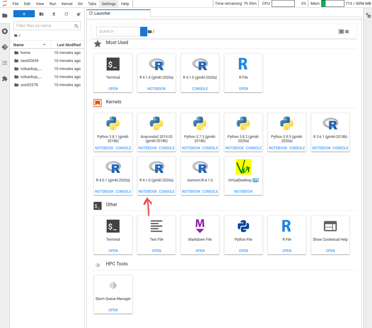
After logging into the NeSI Jupyter lab, open an R (v4.1) notebook.

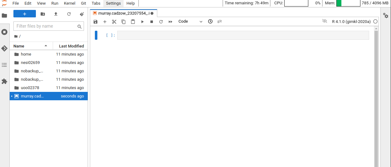
Now that we are ready to start exploring R, we will want to keep a record of the commands we are using in out notebook. Lets first save our new notebook.

Click the File menu and select Save Notebook As and then call it intro_r.ipynb. By convention, notebooks end with the file extension .ipynb.

Overview of the R notebook layout

Here are the main features of the notebook environment:

Some useful keyboard shortcuts:

• To run the current cell: Shift + ENTER
• To insert a new cell above the current cell: ESC + A
• To insert a new cell below the current cell: ESC + B

You are working with R

Although we won’t be working with R at the terminal, there are lots of reasons to. For example, once you have written an RScript, you can run it at any Linux or Windows terminal without the need to start up RStudio. We don’t want you to get confused - Jupyter or RStudio runs R, but R is not RStudio or Jupyter. For more on running an R Script at the terminal see this Software Carpentry lesson.

Getting to work with R: navigating directories

Now that we have covered the more aesthetic aspects of Jupyter notebooks, we can get to work using some commands. We will write, execute, and save the commands we learn in our notebook. First, lets see what directory we are in. To do so, type the following command into the cell:

getwd()

To execute this command, make sure your cursor is on the same line the command is written. Then click the Run (play) button that is just above the first line of your notebook in the header.

In the output, we expect to see the following output*:

[1] "'/scale_wlg_persistent/filesets/home/murray.cadzow/.jupyter/jobs/23207554'"

Since we will be learning several commands, we may already want to keep some short notes in our notebook to explain the purpose of the command. Entering a # before any line in a cell turns that line into a comment, which R will not try to interpret as code. Edit your cell to include a comment on the purpose of commands you are learning, e.g.:

# this command shows the current working directory
getwd()

Exercise: Work interactively in R

What happens when you try to enter the getwd() command in the Console pane?

Solution

You will get the same output you did as when you ran getwd() from the source. You can run any command in the Console, however, executing it from the source script will make it easier for us to record what we have done, and ultimately run an entire script, instead of entering commands one-by-one.

For the purposes of this exercise we want you to be in the directory "~/obss_2021/intro_r". What if you weren’t? You can set your home directory using the setwd() command. Enter this command in your script, but don’t run this yet.

# This sets the working directory
setwd()

You may have guessed, you need to tell the setwd() command what directory you want to set as your working directory. To do so, inside of the parentheses, open a set of quotes. Inside the quotes enter a ~/ which is your home directory for Linux. Next, use the Tab key, to take advantage of the Tab-autocompletion method, to select obss_2021, and intro_r directory. The path in your script should look like this:

# This sets the working directory
setwd("~/obss_2021/intro_r")

When you run this command, the console repeats the command, but gives you no output. Instead, you see the blank R prompt: >. Congratulations! Although it seems small, knowing what your working directory is and being able to set your working directory is the first step to analyzing your data.

Tip: Never use setwd()

Wait, what was the last 2 minutes about? Well, if setting your working directory is something you need to do, you need to be very careful about using this as a step in your script. For example, what if your script is being on a computer that has a different directory structure? The top-level path in a Unix file system is root /, but on Windows it is likely C:\. This is one of several ways you might cause a script to break because a file path is configured differently than your script anticipates. R packages like here and file.path allow you to specify file paths is a way that is more operating system independent. See Jenny Bryan’s blog post for this and other R tips.

Using functions in R, without needing to master them

A function in R (or any computing language) is a short program that takes some input and returns some output. Functions may seem like an advanced topic (and they are), but you have already used at least one function in R. getwd() is a function! The next sections will help you understand what is happening in any R script.

Exercise: What do these functions do?

Try the following functions by writing them in your script. See if you can guess what they do, and make sure to add comments to your script about your assumed purpose.

• dir()
• sessionInfo()
• date()
• Sys.time()

Solution

• dir() # Lists files in the working directory
• sessionInfo() # Gives the version of R and additional info including on attached packages
• date() # Gives the current date
• Sys.time() # Gives the current time

Notice: Commands are case sensitive!

You have hopefully noticed a pattern - an R function has three key properties:

• Functions have a name (e.g. dir, getwd); note that functions are case sensitive!
• Following the name, functions have a pair of ()
• Inside the parentheses, a function may take 0 or more arguments

An argument may be a specific input for your function and/or may modify the function’s behavior. For example the function round() will round a number with a decimal:

# This will round a number to the nearest integer
round(3.14)

[1] 3

Getting help with function arguments

What if you wanted to round to one significant digit? round() can do this, but you may first need to read the help to find out how. To see the help (In R sometimes also called a “vignette”) enter a ? in front of the function name:

?round()

The “Help” tab will show you information (often, too much information). You will slowly learn how to read and make sense of help files. Checking the “Usage” or “Examples” headings is often a good place to look first. If you look under “Arguments,” we also see what arguments we can pass to this function to modify its behavior. You can also see a function’s argument using the args() function:

args(round)

function (x, digits = 0) 
NULL

round() takes two arguments, x, which is the number to be rounded, and a digits argument. The = sign indicates that a default (in this case 0) is already set. Since x is not set, round() requires we provide it, in contrast to digits where R will use the default value 0 unless you explicitly provide a different value. We can explicitly set the digits parameter when we call the function:

round(3.14159, digits = 2)

[1] 3.14

Or, R accepts what we call “positional arguments”, if you pass a function arguments separated by commas, R assumes that they are in the order you saw when we used args(). In the case below that means that x is 3.14159 and digits is 2.

round(3.14159, 2)

[1] 3.14

Finally, what if you are using ? to get help for a function in a package not installed on your system, such as when you are running a script which has dependencies.

?geom_point()

will return an error:

Error in .helpForCall(topicExpr, parent.frame()) :
   no methods for ‘geom_point’ and no documentation for it as a function

Use two question marks (i.e. ??geom_point()) and R will return results from a search of the documentation for packages you have installed on your computer in the “Help” tab. Finally, if you think there should be a function, for example a statistical test, but you aren’t sure what it is called in R, or what functions may be available, use the help.search() function.

Exercise: Searching for R functions

Use help.search() to find R functions for the following statistical functions. Remember to put your search query in quotes inside the function’s parentheses.

• Chi-Squared test
• Student t-test
• mixed linear model

Solution

While your search results may return several tests, we list a few you might find:

• Chi-Squared test: stats::Chisquare
• Student t-test: stats::t.test
• mixed linear model: stats::lm.glm

We will discuss more on where to look for the libraries and packages that contain functions you want to use. For now, be aware that two important ones are CRAN - the main repository for R, and Bioconductor - a popular repository for bioinformatics-related R packages.

Key Points

• R is a powerful, popular open-source scripting language