Data101: From raw data to individual samples files

Overview

Teaching: 0 min
Exercises: 0 min

Questions

• How do we process data from raw reads to individual fastq files?

Objectives

• Check the quality of the data

• Assign reads to individual samples

Developed by: Ludovic Dutoit, Alana Alexander

Adapted from: Julian Catchen, Nicolas Rochette

Background

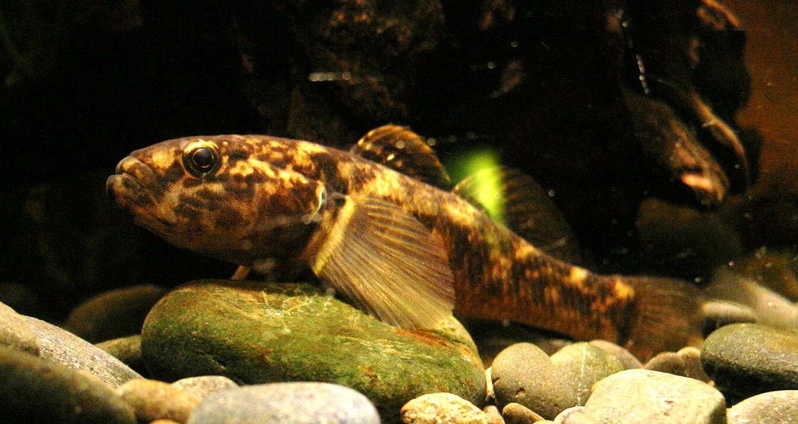
In this tutorial, we will be working with data from Ingram et al. (2020). They sampled common bullies (Gobiomorphus cotidianus; AKA: Lake Fish) from Lake Wanaka and Lake Wakatipu in Aotearoa New Zealand. These fishes look different at different depths, and we found ourselves asking whether those morphological differences were supported by genetic structure. Today we are using a reduced dataset from this paper of 12 fishes, a reasonable size to be able to run all our commands quickly: 6 fishes sampled each from each lake, 3 from each lake at shallow depth, and three coming from deeper depths..

Working with single-end reads

The first step in the analysis of all short-read sequencing data, including RAD-seq data, is separating out reads from different samples that were individually barcoded. This ‘de-multiplexing’ associates reads with the different individuals or population samples from which they were derived.

Getting set up

1. Let’s organise our space, get comfortable moving around, and copy our data :

   • Log into Jupyter at https://jupyter.nesi.org.nz/hub/login. Remember, the second factor is on your phone.
   • You will set up a directory structure on the remote server that will hold your data and the different steps of your analysis. We will start by moving to the gbs/ directory in your working space (~/obss_2021/), so let’s cd (change directory) to your working location:

$ cd ~/obss_2021/gbs

$ pwd

/home/yourname/obss_2021/gbs

NOTE: If you get lost at any time today, you can always cd to your directory with the above command.

The exercise from now on is hands-on: the instructions are here to guide you through the process but you will have to come up with the specific commands yourself. Fear not, the instructors are there to help you and the room is full of friendly faces to help you get through it.

1. We will create more subdirectories to hold our analyses. Be careful that you are reading and writing files to the appropriate directories within your hierarchy. You’ll be making many directories, so stay organized! We will name the directories in a way that corresponds to each stage of our analysis and that allows us to remember where all our files are! A structured workspace makes analyses easier and prevents data from being accidentally overwritten.

Exercise

In gbs/, we will create two directories: lane1 and samples. lane1 will contain the raw data. By the end of the exercise, samples will contain one file per sample with all the reads for that individual.

Solution

$ mkdir lane1 samples

• As a check that we’ve set up our workspace correctly use the ls -R (the ls command with the recursive flag). It should show you the following (./ is a placeholder for ‘current directory’):

./lane1:

./samples:

Exercise

Copy the dataset containing the raw reads to your lane1 directory. The dataset is the file /nesi/project/nesi02659/obss_2021/resources/gbs/lane1.fastq.gz (hint: cp /path/to/what/you/want/to/copy /destination/you/want/it/to/go)

Solution

$ cp /nesi/project/nesi02659/obss_2021/resources/gbs/lane1.fastq.gz lane1/

Examining the data

Let’s have a closer look at this data. Over the last couple of days, you learnt to run FastQC to evaluate the quality of the data. Run it on these files. Load the module first and then run FastQC over the gzipped file. We will help you out with these commands, but bonus question as you work through these: What do the commands module spider, module load, module purge do?

$ module purge
$ module spider fastqc 
$ module load FastQC
$ cd lane1
$ fastqc lane1.fastq.gz

Explanations of this code: module purge get rids of any pre-existing potentially conflicting modules. module spider searches for modules e.g. module spider fastqc looks for a module called fastqc (or something similar!). Once we know what this module is actually called (note: almost everything we do on terminal is case-sensitive) we can use module load to load the module. Finally, we ran fastqc.

You just generated a FastQC report. Use the Jupyter hub navigator tool to follow the path to your current folder (hint: If you’re not quite sure where you are, use pwd in your terminal window. Also, if obss_2021 doesn’t show up in the menu on the left, you might need to also click the littler folder icon just above Name). Once you’ve navigated to the correct folder, you can then double click on a fastqc .html report.

Exercise

What is this odd thing in the per base sequence content from base 7 to 12-13?

Solution

It is the enzyme cutsite. It is identical on all the fragments that were correctly digested by the enzyme before being ligated to a restriction enzyme.

You probably noticed that not all of the data is high quality (especially if you check the ‘Per base sequence quality’ tab!). In general with next generation sequencing, you want to remove the lowest quality sequences and remaining adapters from your data set before you proceed to do anything. However, the stringency of the filtering will depend on the final application. In general, higher stringency is needed for de novo assemblies as compared to alignments to a reference genome. However, low quality data can affect downstream analysis for both de novo and reference-based approaches, producing false positives, such as errant SNP predictions.

We will use the Stacks’s program process_radtags to remove low quality sequences (also known as cleaning data) and to demultiplex our samples. Here is the Stacks manual as well as the specific manual page for process_radtags on the Stacks website to find information and examples.

Exercise

1. Get back into your gbs folder by running cd ../ in the terminal (hint: if you are lost use pwd to check where you are).

2. It is time to load the Stacks module to be able to access the process_radtags command. Find the module and load it (hint: Do for Stacks what we did above for FastQC).

3. You will need to specify the set of barcodes used in the construction of the RAD library. Each P1 adaptor in RAD read starts with a particular DNA barcode that gets sequenced first, allowing data to be associated with individual samples. To save you some time, the barcode file is at: /nesi/project/nesi02659/obss_2021/resources/gbs/lane1_barcodes.txt Copy it to the gbs/ where you currently are. Have a look at the barcodes.

4. Based on the barcode file, can you check how many samples were multiplexed together in this RAD library

5. Have a look at the help online to prepare your process_radtags command. You will need to specify:
   • the restriction enzyme used to construct the library (pstI)
   • the directory of input files (the lane1 directory)
   • the list of barcodes (lane1_barcodes.txt)
   • the output directory (samples)
   • finally, specify that process_radtags needs clean, discard, and rescue reads as options of process_radtags
6. You should now be able to run the process_radtags command from the gbs/ directory using these options. It will take a couple of minutes to run. Take a breath or think about what commands we’ve run through so far.

Solution

### Load the module
$ module load Stacks
### copy the barcodes
$ cp /nesi/project/nesi02659/obss_2021/resources/gbs/lane1_barcodes.txt .
### count barcodes
wc -l lane1_barcodes.txt
### run process_radtags
$ process_radtags  -p lane1/ -o ./samples/ -b lane1_barcodes.txt -e pstI -r -c -q

The process_radtags program will write a log file into the output directory. Have a look in there. Examine the log and answer the following questions:

• How many reads were retained?
• Of those discarded, what were the reasons?
• Use ls -lh samples to have a quick look at the size of the samples files, and make sure all files have data. Well done! Take a break, sit back or help your neighbour, we will be back shortly!

Key Points

• Raw data should always be checked with FastQC.

• Assigning reads to specific samples is called demultiplexing

• process_radtags is the built in demultiplexing tools of Stacks and it includes some basic quality control

De-novo assembly without a reference genome

Overview

Teaching: 0 min
Exercises: 0 min

Questions

• How can we identify genetic variants without a reference genome?

• How to optimise parameters in the Stacks parameter space?

• How to access the full extent of the cluster resources?

Objectives

• Learn to call SNPs without a reference genome and to optimise the procedure

• Learn to run SLURM scripts

Developed by: Ludovic Dutoit, Alana Alexander

Adapted from: Julian Catchen, Nicolas Rochette

Introduction

In this exercise we will identify genetic variants for our 12 common bullies (AKA: Lake fish).

Without access to a reference genome, we will assemble the RAD loci de novo and examine population structure. However, before we can do that, we want to explore the de novo parameter space in order to be confident that we are assembling our data in an optimal way.

The detailed information of the stacks parameter can be found in this explanation.

In summary, Stack (i.e. locus) formation is controlled by three main parameters:

-m : the minimum amount of reads to create a locus (default: 3)

-M : the number of mismatches allowed between alleles of the same locus (i.e. the one we want to optimise)

-n : The number of mismatches between loci between individuals (should be set equal to -M)

-r: minimum percentage of individuals in a population sequences to consider that locus for that population

If that does not make sense or you would like to know more, have a quick read of this explanation from the manual.

Here, we will optimize the parameter -M (description in bold above) using the collaborative power of all of us here today! We will be using the guidelines of parameter optimization outlined in Paris et al. (2017) to assess what value for the -M parameter recovers the highest number of polymorphic loci. Paris et al. (2017) described this approach:

“After putative alleles are formed, stacks performs a search to match alleles together into putative loci. This search is governed by the M parameter, which controls for the maximum number of mismatches allowed between putative alleles […] Correctly setting -M requires a balance – set it too low and alleles from the same locus will not collapse, set it too high and paralogous or repetitive loci will incorrectly merge together.”

As a giant research team, we will run the denovo pipeline with different parameters. The results from the different parameters will be shared using this Google sheet. After optimising these parameters, we’ll be able to use the best dataset downstream for population genetics analyses and to compare it with a pipeline that utilises a reference genome.

In reality, you’d probably do that optimisation with just a few of your samples as running the entire pipeline for several parameters combinations would be something that would consume much resources. But for today, I made sure our little dataset of 12 fishes runs fast enough.

Optimisation exercise

In groups of 2, it is time to run an optimisation. There are three important parameters that must be specified to denovo_map.pl, the minimum stack/locus depth (m), the distance allowed between stacks/loci (M), and the distance allowed between catalog loci (n). Choose which values of M you want to run (M<10), not overlapping with parameters other people have already chosen, and insert them into this google sheet.

If you find most M values already entered in the spreadsheet, we will take the chance to optimise -r, the number of samples that have to be sequenced for a particular locus to be kept it in the dataset (i.e. percentage of non-missing genotypes). Jump onto the second page of that Google sheet and vary -r away from 0.8 (80% of individuals covered while setting -M and -n at 2.

Organise yourself

1. In your gbs/ workspace, create a directory called denovo_output_optimisation for this exercise.

2. Make sure you load the Stacks module (you can check if you have already loaded it using module list)

3. We want Stacks to understand which individuals in our study belong to which population. Stacks uses a so-called population map. The file contains sample names as well as populations. The file should be formatted in 2 columns like this. All 12 samples are recorded in the file at the file path below. Copy it into the gbs/ folder you should currently be in. Note that all the samples have been assigned to a single “dummy” population, ‘SINGLE_POP’, just while we are establishing the optimal value of M in this current exercise.

   /nesi/project/nesi02659/obss_2021/resources/gbs/popmap.txt

Solution

### create folder
$ cd ~/obss2021/gbs/
$ mkdir denovo_output_optimisation
### load Stacks
$ module list
$ module load Stacks
### copy the population map
cp  /nesi/project/nesi02659/obss_2021/resources/gbs/popmap.txt .

Build the denovo_map.pl command

1. Build your Stacks’ denovo_map.pl pipeline program according to the following set of instructions. Following these instructions you will bit by bit create the complete denovo_map.pl command:

• Information on denovo_map.pl and its parameters can be found online. You will use this information below to build your command. You can also use denovo_map.pl --help

• Specify the path to the directory containing your sample files (hint use your samples/ link here!). The denovo_map.pl program will read the sample names out of the population map, and look for associated fastq in the samples directory you specify.

• Make sure you specify this population map to the denovo_map.pl command (use the manual).

• Set the output_denovo_optimisation directory as the output directory.

• Set -M and -n. n should be equal to M, so if you set M at 3, set n at 3.

• Set m at 3, it is the default parameter, we are being explicit here for anyone (including ourselves), reading our code later.

• Set -r to 0.8, unless you are doing the -r optimisation, then set -r to your chosen value

• Finally, use 4 threads (4 CPUs: so your analysis finishes faster than 1!).

• Your command should be ready, try to execute denovo_map.pl (part of the Stacks pipeline).

• Is it starting alright? Good, now Use control + c to stop your command, we’ll be back to it soon

Solution

This command is for someone optimising -M and setting -M at 3

$ denovo_map.pl --samples samples/  --popmap popmap.txt -o denovo_output_optimisation/  -M 3 -n 3 -m 3 -r 0.8 -T 4

Running your first SLURM scipt

Running the commands directly on the screen is not common practice. You now are on a small Jupyter server which has a reserved amount of resources for this workshop and this allows us to run our commands directly. In your day to day activity, you might want to run more than one thing at once or run things for longer or with way more resources than you have on your jupyter account. The way to do this is running your task, also called a job using a SLURM script. The SLURM script (or submission scriptbatch script) accesses all the computing resources that are tucked away from the user. This allows your commands to be run as jobs that are sent out to computing resources elsewhere on Mahuika, rather than having to run jobs your little jupyter server itself. That way you can run many things at once and also use loads more resources. We will use this denovo_map.pl command as a perfect example to run our first job using a batch script.

Your first SLURM script

• copy the example script file into the directory gbs/. The example script is at: /nesi/project/nesi02659/obss_2021/resources/gbs/denovojob.sh

cp /nesi/project/nesi02659/obss_2021/resources/gbs/denovojob.sh .

• Open it with a text editor, have a look at what is there. The first line is #!/bin/bash -e: this is a shebang line that tells the computing environment that language our script is written in. Following this, there are a bunch of lines that start with #SBATCH, which inform the system about who you are, which type of resources you need, and for how long. In other words, your are telling mahuika how big of a computer you want to run that SLURM script.

• For a few of the #SBATCH lines, there are some spaces labelled up like <...> for you to fill in. These spaces are followed by a comment starting with a # that lets you know what you should be putting in there. With this information, fill in your SLURM script. These are the resources you are requesting for this SLURM script.

• Once you are done, save it. Then run it using:

sbatch denovojob.sh

You should see Submitted batch job and then a random ID number.

You can check what the status of your job is using:

squeue -u <yourusername>

If your job is not listed in squeue. It has finished running. It could be have been successful or unsuccessful (i.e. a dreaded bug), but if it is not in the queue, it has run. What would have printed to your screen has instead printed into the file denovo.log. If your job finished running immediately, go check that file to find a bug. If your job appear in the queue for more than 10s, you proably set it up correctly, sit back, it is probably time for a break.

We used a few basic options of sbatch, including time, memory, job names and output log file. In reality, there are many, many, more options. Have a quick look at sbatch --help out of interest. NeSI also has its own handy guide on how to submit a job here.

It is worth noting that we quickly test ran our command above before putting it in a job. This is a very important geek hack. Jobs can stay in the queue not running for some amount of time. If they fail on a typo, you’ll have to start again. Quickly testing a command before stopping it using ctrl + c is a big time saver.

Analysing the result of our collective optimisation

Analysing the main output files

Now that your execution is complete, we will examine some of the output files. You should find all of this info in denovo_output_optimisation/

• After processing all the individual samples through ustacks and before creating the catalog with cstacks, denovo_map.pl will print a table containing the depth of coverage of each sample. Find this table in output_denovo_optimisation/denovo_map.log: what were the depths of coverage?

• Examine the output of the populations program in the file populations.log inside your output_denovo_optimisation folder (hint: use the less command).

• How many loci were identified?

• How many variant sites were identified?

• Enter that information in the collaborative Google Sheet

• How many loci were filtered?

• Familiarize yourself with the population genetics statistics produced by the populations component of stacks populations.sumstats_summary.tsv inside the output_denovo_optimisation folder

• What is the mean value of nucleotide diversity (π) and FIS across all the individuals? [hint: The less -S command may help you view these files easily by avoiding the text wrapping]

Congratulations, you went all the way from raw reads to genotyped variants. We’ll have a bit of a think as a class compiling all this information.

Key Points

• -M is the main parameter to optimise when identifying variants de-novo using Stacks

• Optimisation can often be performed with a subset of the data

• SLURM scripts are the way to harvest the cluster’s potential by running jobs

Assembly with a reference genome

Overview

Teaching: 0 min
Exercises: 0 min

Questions

• How do we identify genetic variants if we have a reference genome?

Objectives

• Learn to call SNPs with a reference genome

• Practice running SLURM scripts

• Practice mapping reads to a reference genome

Developed by: Ludovic Dutoit, Alana Alexander

Adapted from: Julian Catchen, Nicolas Rochette

Introduction

Obtaining an assembly without a reference genome is easy and possible. However, having a reference genome allows us to avoid several issues. We do not have to make assumptions about the “best” value for the -M parameter, and we reduce the risk of collapsing different loci together (“lumping”) or separating one “real” locus into several “erroneous loci” (“splitting”). Studies have demonstrated that having some kind of reference genome is the single best way you can improve GBS SNP calling (see for example Shafer et al. 2016). Using a related species genome might be good enough in several cases too (but it sometimes depends on your application).

The stacks pipeline for samples with a reference genome is ref_map.pl. It skips the creation of loci and the catalog steps as reads belong to the same stack/locus if they map to the same location of the reference genome. This means we don’t have to rely on assumptions derived from genetic distances (-M and -n of denovo_map.pl) about whether reads belong to the same locus or not.

We don’t have a genome for our common bullies yet. Instead, we will map the reads to the catalog of loci that stacks as created for one of our denovo runs. You would never do that in the real world, but that gives us a chance to run the ref_map.pl pipeline.

Map your samples to the reference

Organise yourself

1. Get back to gbs/

2. In the folder gbs/ create an output folder for this analysis, refmap_output/ as well as the folder samples_mapped

3. Copy the reference catalog below that we will use as a pretend reference genome to inside the gbs/ folder you should currently be in.

/nesi/project/nesi02659/obss_2021/resources/gbs/reference_catalog.fa

Have a quick look inside the first few lines of reference_catalog.fa using head -n 10 reference_catalog.fa. It contains each loci identified in the denovo approach as a complete sequence.

Solution

$ mkdir samples_mapped
$ mkdir refmap_output
$ cp  /nesi/project/nesi02659/obss_2021/resources/gbs/reference_catalog.fa .
$ head -n 10 reference_catalog.fa  

It is about time to remind ourselves about a couple of mapping softwares. BWA is a piece of software that is commonly used for mapping. bwa mem is the ideal algorithm to align our short reads to the pretend reference genome. We will also use Samtools, a suite of tools designed to interact with the sam/bam alignment format (i,e, sorting, merging, splitting, subsetting, it is all there).

Load the software

Identify the 2 modules you need for bwa and Samtools and load them. You need to index your reference genome. This is basically creating a map of your genome so that BWA can navigate it extra fast instead of reading it entirely for each read. Use bwa index YOURGENOME.fa for that.

Solution

$ module spider BWA
$ module load BWA
$ module spider samtools
$ module load SAMtools
$ bwa index reference_catalog.fa  

Well done, we are now ready to do the mapping!

Mapping command

For each sample, we will now take the raw reads and map them to the reference genome, outputting a sorted .bam file inside the folder samples_mapped.

For a single sample, the command looks like this:

$ bwa mem -t 4 reference_catalog.fa  samples/MYSAMPLE.fq.gz   |  samtools view -b | samtools sort --threads 4 > samples_mapped/MYSAMPLE.bam 

Explanations: bwa mem uses 4 threads to align samples/MYSAMPLE.fq.gz to the reference catalog. The output is piped using the | symbol into the next command instead of being printed to the screen. samtools view creates a bam file using -b. That bam output is piped into the samtools sort command before finally being outputted as a file using > into samples_mapped.

Now this is all well and good, but we don’t want to do it manually for each sample. The for loop below is doing it for all samples by going through all the samples/*.fq.gz files.

This is the chunkiest piece of code today. So no problem if you don’t soak it all in. If you are in a classroom right now, we’ll probably look at loops together. Otherwise, you could have a look at how they work here.

$ for filename in samples/*fq.gz
	do base=$(basename ${filename} .fq.gz)
 	echo $base
  	bwa mem -t 4 reference_catalog.fa  samples/${base}.fq.gz | samtools view -b | samtools sort --threads 4 > samples_mapped/${base}.bam 
 done

Explanations: for each filename in the folder ‘samples’ that ends with .fq.gz, extract only the prefix of that filename: samples/PREFIX.fq.gz with the basename function. Print the filename we are currently working with using echo. Use the bwa + samtools mapping explained above, using the base name to output a file PREFIX.bam.

Well done, we only have ref_map.pl to run now.

Run the ref_map pipeline

ref_map.pl has fewer parameters since the mapping takes care of many of the steps from denovo_map.pl, such as the creation of loci for each individual before a comparison of all loci across all individuals. ref_map.pl uses the mapped files to identify the variable positions.

build your ref_map.pl command

Use the online help to build your refmap.pl command. you can also check ref_map.pl --help.
• Unlike in the previous exercise, ask for 2 threads

• Specify the path to the input folder samples_mapped/

• Specify the path to the output folder refmap_output/

• Specify the path to the population map. We will be able to use the same popmap as for the denovo analysis, since we are using the same samples.

• We only want to keep the loci that are found in 80% of individuals. This is done by passing specific arguments to the populations software inside Stacks.

• Is your command ready? Run it briefly to check that it starts properly, once it does stop it using ctrl + c, we’ll run it as a job.

Solution

ref_map.pl -T 2 --samples samples_mapped/  -o refmap_output/ --popmap popmap.txt -r 0.8

Create the job file

• Time to put that into a job script. You can use the job script from the last exercise as a template. We will simply make a copy of it under a different name. In practice, we often end up reusing our own scripts. Let’s copy the denovojob.sh into a new refmapjob.sh:

cp denovojob.sh refmapjob.sh

• Open refmapjob.sh using a text editor. Adjust the job name, adjust the number of threads/cpus to 2, adjust the running time to 10min, and the job output to refmap.log instad of denovo.log. Most importantly, replace the denovo_map.pl command with your ref_map.pl command.

• Save it, and run the job: sbatch refmapjob.sh

That should take about 5 minutes. Remember you can use squeue -u <yourusername> to check the status of the job. Once it is not there anymore, it has finished. This job will write out an output log called refmap_output/refmap.log that you can check using less.

Analyse your results

## Looking into the output
• Examine the output of the populations program in the file ref_map.log inside your refmap_output folder. (hint: use the less command).

• How many SNPs were identified?

• Why did refmap.pl run faster than denovo_map.pl ?

Well done, you now know how to call SNPs with or without a reference genome. It is worth re-iterating that even a poor-quality reference genome should improve the quality of your SNP calling by avoiding lumping and splitting errors. But beware of some applications. Inbreeding analyses are one example of applications that are sensitive to the quality of your reference genome.

Only one thing left, the cool biology bits.

Key Points

• Reference genomes, even of poor quality or from a related species are great for SNP identification

• Reference-based SNP calling takes the guess work of distance between and within loci away by mapping reads to individual location within the genome

Population genetics analyses

Overview

Teaching: 0 min
Exercises: 0 min

Questions

• How do I navigate filtering my SNPs?

• How can I quickly visualise my data?

Objectives

• Learn to navigate SNP filtering using Stacks

• Learn basic visualisation of population genetic data

Developed by: Ludovic Dutoit, Alana Alexander

Adapted from: Julian Catchen, Nicolas Rochette

Introduction

In this exercise, we’ll learn about filtering the variants before performing two population genetics structure analyses. We’ll visualise our data using a Principal Component Analysis (PCA), and using the software Structure.

Part 1: Data filtering

Getting the data

We will work with the best combination of parameters identified from our collective optimisation exercise.

Obtain the optimised dataset

• Get back to the gbs/ folder

• The optimised dataset can be optained from the link below, use the -r parameter of the cp command. That stands for recursive and allow you to copy folders and their content. /nesi/project/nesi02659/obss_2021/resources/gbs/denovo_final/

• We’ll also copy a specific population map that is encoding the 4 different possible populations ( 2 lakes x 2 depths). That population map is at /nesi/project/nesi02659/obss_2021/resources/gbs/complete_popmap.txt.

• Once you copied it, have a quick look at the popmap using less

Solution

$ cp -r /nesi/project/nesi02659/obss_2021/resources/gbs/denovo_final/ .
$ cp /nesi/project/nesi02659/obss_2021/resources/gbs/complete_popmap.txt .
$ less complete_popmap.txt  # q to quit

Filtering the Data

You might have noticed that we have not really looked at our genotypes yet. Where are they? Well, we haven’t really picked the format we want them to be written in yet. The last module of Stacks is called populations. populations allows us to export quite a few different formats directly depending on which analyses we want to run. Some of the formats you might be familiar with are called .vcf .phylip or .structure (see File Output Options). The populations module also allows filtering of the data in many different ways as can be seen in the manual. populations is run at the end of ref_map.pl or denovo_map.pl, but it can be re-run as a separate step to tweak our filtering or add output files.

SNP filtering is a bit of a tricky exercise that is approached very differently by different people. Here are my three pieces of advice. Disclaimer: This is just how I approach things, other people might disagree.

1. A lot of things in bioinformatics can be seen in terms of signal to noise ratio. Filtering your variants can be seen as maximising your signal (true genotypes) while reducing your noise (erroneous SNPs, missing data).

2. Think of your questions. Some applications are sensitive to data filtering, some are less sensitive. Some applications are sensitive to some things but not others. They might be sensitive to missing data but not the absence of rare variants. In general, read the literature and look at their SNP filtering.

3. Don’t lose too much time hunting the perfect dataset, try creating one that can answer your question. I often see people that try optimising every single step of the pipeline before seeing any of the biological outputs. I find it is often easier to go through the whole pipeline with reasonable guesses on the parameters to see if it can answer my questions before going back if needed and adapting it. If you then need to go back, you’ll be a lot more fluent with the program anyway, saving yourself a lot of time.

Right, now that we went through this, let’s create our populations command using the manual.

Building the populations command

• Specify denovo_final/ as the path to the directory containing the Stacks files.

• Also specify denovo_final/ as the output folder

• Specify the population map that you just copied

• Specify the minimum proportion number of individuals covered to 80%

• In an effort to keep statistically independent SNPs, specify that only one random SNP per locus should be outputted.

• Make sure to output a structure file and a .vcf file as well. We might be coming back to that .vcf file later today.

Solution

$ populations -P denovo_final/ -O denovo_final/ -M complete_popmap.txt  -r 0.8 --write-random-snp  --structure --vcf

How many SNPs do you have left?

Creating a white list

In order to run a relatively quick set of population genetics analyses (i.e. for today), we will save a random list of 1000 loci into a file and then ask populations to only output data from these loci. Such a list is named a white list, intuitively the opposite of a black list. We can create a random white list by using the shell given a list of catalog IDs from the output ofpopulations. We will use the file denovo_final/populations.sumstats.tsv. Quickly check it out using:

$ less -S denovo_final/populations.sumstats.tsv # use q to quit

Create the white list.

With the help of the instructions below, use the cat, grep, cut, sort, uniq, shuf, and head commands to generate a list of 1,000 random loci. Save this list of loci as whitelist.txt, so that we can feed it back into populations. This operation can be done in a single shell command. That sounds challenging, but the instructions below should help you create one command with several pipes to create that whitelist.txt file. The idea of a pipe is to connect commands using | e.g. command 1 | command 2 outputs the content of command 1 into command 2 instead of outputting it to the screen.

At each step, you can run the command to see that it is outputting what you want, before piping it into the next step. Remember, you can access your last command in the terminal by using the up arrow key.

• First, use cat to concatenate denovo_final/populations.sumstats.tsv.

• Then, stream it into the next command using a |.

• Use the command grep with -v to exclude all headers (i.e. -v stands for exclude, we want to exclude all the lines with “#”).

• Add another | and select the first column with cut -f 1

• Then using two more pipes, use sort before using uniq. uniq will collapse succesive identical lines into single lines, so that you have one line per locus. Lucky us, those two commands don’t require any arguments. We have to use sort first to make sure identical lines are next to each other, otherwise they won’t collapse.

• Now try adding shuf which will mix all these lines all over.

• Select the first one thousand lines with head -n 1000

• Well done, redirect the output of head into the file whitelist.txt. (hint: use “>” to redirect into a file). Do not worry if you get an error similar to the following about the shuf command: write error: Broken pipe, it is simply because head stops the command before the end.

• You did it! If you are new to bash, I am sure writing this command seemed impossible on Monday, so take a minute to congratulate yourself on the progress made even if you required a little help.

Solution

cat denovo_final/populations.sumstats.tsv | grep -v "#" | cut -f 1 | sort | uniq | shuf | head -n 1000 > whitelist.txt

Execute populations with the white list

Now we will execute populations again, this time feeding back in the whitelist you just generated. Check out the help of populations to see how to use a white list. This will cause populations to only process the loci in the whitelist.txt.

The simple way to do this is to start with the same command than last time:

$ populations -P denovo_final/ -O denovo_final/ -M complete_popmap.txt  -r 0.8 --write-random-snp  --structure --vcf

with one modification:

• Specify the whitelist.txt file that you just generated as a white list.

• Ready? Hit run!

Solution

populations -P denovo_final/ -O denovo_final/ -M complete_popmap.txt  -r 0.8 --write-random-snp  --structure --vcf -W whitelist.txt

• Did you really need to specify -r?

• What about --write-random-snp, did we need it?

We’ve run commands to generate the structure file two times now, but how many structure files are there in the stacks directory? Why?

If you wanted to save several different vcf and structure files generated using different populations options, what would you have to do?

Part 2: Population genetics analyses

To recap: in this exercise we are using common bullies (Gobiomorphus cotidianus; AKA: Lake Fish) sampled from Lake Wanaka and Lake Wakatipu in Aotearoa New Zealand. These fishes look different at different depths, and we found ourselves asking whether those morphological differences were supported by genetic structure. We’ve got a reduced dataset of 12 fishes, a reasonable size to be able to run all our commands quickly: 6 fishes sampled each from each lake, 3 from each lake at shallow depth, and 3 coming from deeper depths.

Principal Component analysis (PCA)

Let’s get organised

• Create a pca/ folder inside your gbs/ folder

• Copy the .vcf/ file inside denovo_final inside pca/ (if you’re not sure what it is called, remember it ends with .vcf)

• Get inside the pca folder to run the rest of the analyses

Solution

$ mkdir pca
$ cp denovo_final/*.vcf pca/
$ cd pca

For the rest of the exercise, we will use R. You can run R a few different ways, you can use it from within the unix terminal directly or by selecting a R console or an R notebook from the jupyter launcher options. As our R code is relatively short, we’ll save ourselves the pain of clicking around and we’ll launch R from within the terminal. If you want to go to the R console or notebook, feel free to do so but make sure you select R 4.1.0.

$ module load R-bundle-Bioconductor/3.13-gimkl-2020a-R-4.1.0
$ R

You are now running R, first off, let’s load the pcadapt package.

> library("pcadapt") 

Let’s read in our vcf and our popmap as a metadata file to have population information

> vcf <- read.pcadapt("populations.snps.vcf", type = "vcf")
> metadata <- read.table("../complete_popmap.txt",h=F)
> colnames(metadata) <- c("sample","pop")

Finally, let’s run the PCA.

> pca <- pcadapt(input = vcf, K = 10) # computing 10 PC axes
> png("pca.png") # open an output file
> plot(pca, option = "scores",pop=metadata$pop)
> dev.off() # close the output file

• Use the navigator on the left to go find the file pca.png inside the folder pca/

• What do you see, is there any structure by lake? by depth?

We really did the simplest PCA, but you can see how it is a quick and powerful to have an early look at your data. You can find a longer tutorial of pcadapt here.

Structure

Our goal now is to use our dataset in Structure, which analyzes the distribution of multi-locus genotypes within and among populations in a Bayesian framework to make predictions about the most probable population of origin for each individual. The assignment of each individual to a population is quantified in terms of Bayesian posterior probabilities, and visualized via a plot of posterior probabilities for each individual and population.

A key user defined parameter is the hypothesized number of populations of origin which is represented by K. Sometimes the value of K is clear from from the biology, but more often a range of potential K-values must be explored and evaluated using a variety of likelihood based approaches to decide upon the ultimate K. In the interests of time we won’t be exploring different values of K here, but this will be a key step for your own datasets. We’ll just see what we get with K = 4 as we have up to 4 different populations. In addition, Structure takes a long time to run on the number of loci generated in a typical RAD data set because of the MCMC algorithms involved in the Bayesian computation. Therefore we therefore will continue to use the random subset of loci in our whitelist.txt file. Despite downsampling, this random subset contains more than enough information to investigate population structure.

Run structure

• Leave R using ctrl+z Get back in the gbs/ directory

• Create a structure directory

• Copy the denovo_final/populations.structure file inside the structure/ directory

• Get inside the structure directory

• Edit the structure output file to remove the entire comment line (i.e. first line in the file, starts with “#”).

• So far, when we’ve gone to run programs, we’ve been able to use module spider to figure out the program name, and then module load program_name to get access to the program and run it. Do this again to load structure.

• The parameters to run structure (with value of K=4) have already been prepared, you can find them here: /nesi/project/nesi02659/obss_2021/resources/gbs/mainparams and /nesi/project/nesi02659/obss_2021/resources/gbs/extraparams. Copy them into your structure directory as well.

• Run structure by simply typing structure

• Do you see WARNING! Probable error in the input file? In our mainparams file it says that we have 1000 loci, but due to filters, it is possible that the populations module of Stacks actually output less than the 1000 loci we requested in whitelist.txt. In the output of populations.log in your denovo_final/ directory, how many variant sites remained after filtering? This is the number of loci actually contained in your structure file. You will need to adjust the number of loci in the mainparams file to match this exact Stacks output.

I could have saved you that bug, but it is a very common one and it is rather obscure, so I wanted to make sure you get to fix it here for the first time rather than spending a few hours alone on it.

Solution

$ mkdir structure
$ cp denovo_final/populations.structure structure
$ cd structure

Use nano or a text editor of your choise to remove the first line of the populations.structure file.

$ module spider structure
$ module load Structure
$ cp /nesi/project/nesi02659/obss_2021/resources/gbs/mainparams .
$ cp /nesi/project/nesi02659/obss_2021/resources/gbs/extraparams .
structure

Structure Visualisation

Now that we you ran structure successfully. It is time to visualise the results. We will do that in R. Open R using either a launcher careful to open R 4.1.0 or by typing R. Then use the code below to generate a structure plot.

> library("pophelper")# load plotting module for structure 
> data <- readQ("populations.structure.out_f",filetype = "structure",indlabfromfile=TRUE) # Don't worry about the warning messages
> metadata <- read.table("../complete_popmap.txt",h=F)
> rownames(data[[1]]) <- metadata[,1]
> plotQ(data,showindlab = TRUE,useindlab=TRUE,exportpath=paste(getwd(),"/",sep=""))  

That should create a structure image populations.structure.out_f.png in your structure folder. Use the path navigator on the left to reach your folder to be able to visualise the picture by double-clicking on it. Each column is a sample. Individuals are assigned to up to 4 different clusters to maximise the explained genetic variance. These clusters are represented in 4 different colours.

• Do you see a similar structuring as in the PCA analysis?

Congrats, you just finished our tutorial for the assembly of RAD-Seq data. Here are a few things you could do to solidify your learning from today.

Extra activities

• You could play a bit with the parameters of plotQ() at http://www.royfrancis.com/pophelper/reference/readQ.html to make a prettier structure plot.

• You could spend a bit of time going through and making sure you understand the set of steps we did in our exercises.

• You could try running this set of analyses on a de novo dataset with a different value of -M to see if it makes any difference, or on the reference-based mapping dataset.

• You could have a look at this tutorial. It is a small tutorial I wrote previously that goes over a different set of population genetics analyses in R. You could even try reproducing it using the vcf you generated above. The vcf for the set of analyses presented in that code can be downloaded here should you want to download it.

Key Points

• SNP filtering is about balancing signal vs noise

• Populations is the stacks implemented software to deal with filtering of SNPs

• Principal component analysis (PCA) and Structure are easy visualisation tools for your samples